Some Recent Results on Minibatch Markov Chain Monte Carlo Methods

I have recently been working on minibatch Markov chain Monte Carlo (MCMC) methods for Bayesian posterior inference. In this post, I’d like to give a brief summary of what that means and mention two ICML papers (from 2011 and 2014) that have substantially influenced my thinking.

When we say we do “MCMC for Bayesian posterior inference,” what this typically means is that we have some dataset \(\{x_1,x_2,\ldots,x_N\}\) and a parameter of interest \(\theta \in \mathbb{R}^K\) for some \(K \ge 1\). The posterior distribution \(f(\theta)\) we wish to estimate (via sampling) is

You’ll notice that we assume the data is conditionally independent given the parameter. In many cases, this is unrealistic, but most of the literature assumes this for simplicity.

After initializing \(\theta_0\), the procedure for sampling the posterior on step \(t+1\) is:

• Draw a candidate \(\theta'\)
• Compute the acceptance probability (note that the denominators of \(f\) cancel out):

• Draw \(u \sim {\rm Unif}[0,1]\), and accept if \(u < P_a\). This means setting \(\theta_{t+1} = \theta'\). Otherwise, we set \(\theta_{t+1} = \theta_t\) and repeat this loop. This tripped me up earlier. Just to be clear, we generate a sample \(\theta\) every iteration, even if it is a repeat of the previous one.

This satisfies “detailed balance,” which roughly speaking, means that if one samples long enough, one will arrive at a stationary distribution matching the posterior, though a burn-in period and/or only using samples at regular intervals is often done in practice. The resulting collection of (correlated!) samples \(\{\theta_1, \theta_2, \ldots, \theta_T\}\) for large \(T\) can be used to compute the value of \(p(\theta \mid x_1,\ldots,x_N)\). Let’s consider a very simple example. Say \(\theta\) can take on three values: \(A\), \(B\), and \(C\). If our sampled set is \(\{A,B,B,C\}\), then since \(B\) appears two times out of four, we have \(p(\theta = B \mid x_1,\ldots,x_N) = 2/4\). The other two probabilities would naturally have \(1/4\) each according to the samples.

One issue with the standard procedure above is that in today’s big data world with \(N\) on the order of billions, it is ridiculously expensive to compute \(P_a\) because that involves determining all \(N\) of the likelihood factors. Remember, this has to be done every iteration! Doing all this just to get one bit of data (whether to accept or not) is not a good tradeoff. Hence, there has been substantial research on how to perform minibatch MCMC on large datasets. In this case, rather than use all \(N\) data points, we just use a subset \(n \ll N\) of points each iteration. This approximates the target distribution. The downside? It no longer satisfies detailed balance. (I don’t know the details on why, and it probably involves some complicated convergence studies, but I am willing to believe it.)

Just to be clear, we are focusing on getting a distribution, not a point estimate. That’s the whole purpose of Bayesian estimation! A distribution means we need a full probability function that sums to one and is non-negative; if \(\theta\) is one or two dimensional, we can easily plot the posterior estimate (I provide an example of this later in this post). A point estimate means finding one value of \(\theta^*\), usually the “best”, which we commonly express as the maximum likelihood estimate \(\theta^* = \theta_{\rm MLE}\).

All right, now let’s briefly discuss two papers that tackle the problem of minibatch MCMC.

Bayesian Learning via Stochastic Gradient Langevin Dynamics

This paper appeared in ICML 2011 and proposes using minibatch update methods for Bayesian posterior inference, with a concept known as Langevin Dynamics to inject the correct amount of noise into parameter updates so that the set of sampled parameters converges to the posterior, and not just a mode. To make the distinction clear, let’s see how we can use minibatch updates to converge to a mode — more specifically, the maximum a posteriori estimate. The function \(f\) we are trying to optimize is listed above. So … we just use stochastic gradient ascent! (We are ascending, not descending, because \(f\) is a posterior probability, and we want to make its values higher.) This means the update rule is as follows: \(\theta_{t+1} = \theta_t + \alpha_t \nabla f(\theta_t)\). Plugging in \(f\) above, we get

where \(\epsilon_t\) is a sequence of step sizes.

The above is a stochastic gradient ascent update because we use \(n \ll N\) terms to approximate the gradient value, which is why I inserted an approximation symbol (\(\approx\)) in the underbrace. Because we only use \(n\) terms, however, we must multiply the summation by \(N/n\) to rescale the value appropriately. Intuitively, all those terms in that summation are negative since they’re log probabilities. If we use \(n\) instead of \(N\) terms, that summation is strictly smaller in absolute value. So we must rescale to make the value on the same order of magnitude. Another way of putting it is that the subsampled sum will be an unbiased estimator of the full-batch quantity.

What’s the problem with the above for Bayesian posterior inference? It doesn’t actually do Bayesian posterior inference. The above will mean \(\theta\) converges to a single value. We instead want a distribution. So what can we do? We can use Langevin Dynamics, meaning that (for the full batch case) our updates are:

A couple of things are worth noting:

• We use all \(N\) terms in the summation, so the gradient is in fact exact.
• The injected noise \(\eta_t\) means the \(\theta_{t}\) values will “bounce around” to approximate a distribution and not converge to a single point.
• The \(\epsilon\) is now constant instead of decreasing, and is balanced so that the variance of the injected noise matches that of the posterior.
• We use \(x_i\) instead of \(x_{ti}\) as we did earlier. The only difference is that the \(t\) indicates the randomness in the minibatch. It does not mean that \(x_{ti}\) is one scalar element of a vector. In other words, both \(x_i\) and \(x_{ti}\) are in \(\mathbb{R}^k\) for some \(k\).

For simplicity, the above assumes that \(\eta_t \in \mathbb{R}\). In the general case, these should be multivariate Gaussians, with covariance \(\epsilon I\).

The problem with this, of course, is the need to use all \(N\) points. So let’s use \(n \ll N\) points, and we have the following update:

where now, we need \(\epsilon_t\) to vary and decrease towards zero. The reason for this is that as the step size goes to zero, the corresponding (expensive!) Metropolis-Hastings test has rejection rates that decrease to zero. Thus, we can omit the test to make the algorithm computationally cheap.

Fortunately, the authors show that despite how the noise goes to zero, the set of samples from SGLD will indeed converge to the correct posterior distribution, just as with “normal” (i.e., full-batch) Langevin Dynamics noise.

Austerity in MCMC Land: Cutting the Metropolis-Hastings Budget

This paper appeared in ICML 2014, and is also about minibatch MCMC. Here, instead of relying on simulating the physics of the system (as was the case with Stochastic Gradient Langevin Dynamics), they propose reformulating the standard MCMC method with the standard MH test into a sequential hypothesis test. To frame this, they take the log of both sides of the acceptance inequality:

In the first step we also dropped the initial “min” because if the “1” case applies, we will always accept. In the last step we divide both sides by \(N\). What is the purpose of this? The above is equivalent to the original MH test. But the right hand side depends on all \(N\) data points, so what happens if we compute the right hand side using \(n \ll N\) points?

This is the heart of their test. They start out by using a small fraction of the points and compute the right hand side. If the proposed \(\theta'\) element is so out of whack, then even with just \(n\) points, we should already know to reject it. (And a similar case holds if \(\theta'\) is really good.) If we cannot tell whether to accept or reject \(\theta'\) with some specified confidence threshold, then we increase the minibatch size and test again. Their acceptance test relies on the Central Limit Theorem and the Student-t distribution. The details are in the paper, but the main idea is straightforward: increasing the number of samples increases our certainty as to whether we accept or reject, and we can generally make these decisions with far fewer than \(N\) samples.

What’s the downside of their algorithm? In the worst case, we might need the entire data in one iteration. This may or may not be a problem, depending on the particular circumstances.

Their philosophy runs deeper than what the above says. Here’s a key quote:

We advocate MCMC algorithms with a “bias-knob”, allowing one to dial down the bias at a rate the optimally balances error due to bias and variance.

One other algorithm that adheres to this strategy? Stochastic Gradient Langevin Dynamics! (Not coincidentally, Professor Max Welling is a co-author on both papers.) Side note: the reason why SGLD is biased is because it omits the Metropolis-Hastings test. The reason why this algorithm (Adaptive Sampling) is biased is because it makes decisions based on a fraction of the data. So both are biased, but for slightly different reasons.

Putting it All Together: A Code Example

In order to better understand the two papers described above, I wrote some Python code to run SGLD and adaptive sampling. I also implemented the standard (full-batch) MCMC method for a baseline.

I tested using the experiment in Section 5.1 of the SGLD paper. The parameter is 2-D, \(\theta = (\theta_1,\theta_2)\), and the parameter/data generation process is

and

I’ve pasted all my Python code here. If you put this together in a Jupyter notebook, it should work correctly. If your time is limited, feel free to skip the code and go straight to the output. The code is here mainly for the benefit of current and future researchers who might want a direct implementation of the above algorithms.

The first part of my code imports the necessary libraries and generates the data according to my interpretation of their problem. I am generating 500 points here, whereas the SGLD paper only used 100 points.

# Import necessary libraries
import numpy as np
import matplotlib.pyplot as plt
%matplotlib inline
from scipy.stats import t

# Generate the data according to Section 5.1 of "Bayesian Learning via SGLD."
N = 500 # The number of data points; we reference this frequently later.
sigma1_sq = 10
sigma2_sq = 1
sigmax_sq = 2
theta1 = 0
theta2 = 1

# Generate the data X. The np.random.normal(...) requires STD (not VAR).
X = np.zeros(N)
for i in xrange(N):
    u = np.random.random()
    if (u < 0.5):
        X[i] = np.random.normal(theta1, np.sqrt(sigmax_sq))
    else:
        X[i] = np.random.normal(theta1+theta2, np.sqrt(sigmax_sq))

Next, I define a bunch of functions that I will need for the future. The most important one is the log_f function, which returns the log of the posterior. (Implementing this correctly requires filling in some missing mathematical details that follow from the formulation of multivariate Gaussian densities.)

def log_f(theta, X):
    """
    The function 'f' is the posterior:
    
        f(\theta) \propto p(\theta) * \prod_{i=1}^N p(x_i | \theta)
    
    This method returns the *log* of f(\theta), for obvious reasons.
    X is assumed to be of shape (n,) so we reshape it into (n,1) for vectorization.
    We use [0,0] since we get a float in two lists, [[x]], so calling [0,0] gets x.
    """
    scale = N / float(len(X))
    
    inverse_covariance = np.array([[0.1,0],[0,1]])
    prior_constant = 1.0 / (2*np.pi*np.sqrt(10))
    prior = np.log(prior_constant) - 0.5*(theta.T).dot(inverse_covariance).dot(theta)
    
    X_all = X.reshape((len(X),1))
    ll_constant = (1.0 / (4*np.sqrt(np.pi)))
    L = ll_constant * (np.exp(-0.25*(X_all-theta[0])**2) + np.exp(-0.25*(X_all-(theta[0]+theta[1]))**2))
    log_likelihood = np.sum(np.log(L)) * scale
    
    assert not np.isnan(prior + log_likelihood)
    return (prior + log_likelihood)[0,0]
    
    
def grad_f(theta, X):
    """ Computes gradient of log_f by finite differences. X is (usually) a mini-batch. """
    eps = 0.00001
    base1 = np.array([[eps],[0]])
    base2 = np.array([[0],[eps]])
    term1 = log_f(theta+base1, X) - log_f(theta-base1, X)
    term2 = log_f(theta+base2, X) - log_f(theta-base2, X)
    return np.array([[term1],[term2]])/(2*eps)
    
 
def get_delta(theta_c, theta_p, X):
    """
    Compute the delta term, so we use min{1, exp(\Delta')} for standard MCMC.
    
    theta_c is the *current* theta that we may "leave" (old theta)
    theta_p is the *proposed* theta that we might accept (new theta)
    """
    loss_old = log_f(theta_c, X)
    loss_new = log_f(theta_p, X)
    assert not np.isnan(loss_new - loss_old)
    return loss_new - loss_old


def get_noise(eps):
    """ Returns a 2-D multivariate normal vector with covariance matrix = diag(eps,eps). """
    return (np.random.multivariate_normal(np.array([0,0]), eps*np.eye(2))).reshape((2,1))


def log_f_prior(theta):
    """
    Returns log p(\theta), the prior. Remember, it's returning LOGS. Don't take logs again! 
    This is only used for the adaptive sampling method's hypothesis testing.
    """
    cov_inv = np.array([[0.1,0],[0,1]])
    return np.log(1.0/(2*np.pi*np.sqrt(10))) - 0.5*(theta.T).dot(cov_inv).dot(theta)
        
        
def approximate_mh_test(theta_c, theta_p, m1, X, mu_0, eps_tolerance):
    """
    Implements the adaptive sampling method. Each time we call this, we shuffle the data.
    
    theta_c is the current \theta
    theta_p is the proposed \theta
    m1 is the starting minibatch size
    X is the full data matrix
    mu_0 is equation 2 from "Cutting the MH" paper, pre-computed
    eps_tolerance is for deciding whether delta is small enough
    
    Returns ('accept', 'size'), where 'accept' is a boolean to indicate if we accept or not,
        while 'size' is the size of the mini-batch we sampled (generally a multiple of m).
    """
    
    accept = False
    done = False
    first_iteration = True
    n = 0
    m2 = m1 # We'll increment by the same amount as 'm1', the starting size.
    
    # Shuffle at beginning so we can do X_mini = X[:n]
    index = np.random.permutation(N)
    X = X[index]

    while not done:
        
        # Draw mini-batch without replacement, but keep using same indices we've used.
        # Note that we can have a special case for the first minibatch.
        if first_iteration:
            size = np.min([m1, N])
            first_iteration = False
        else:
            size = np.min([m2, N-n])
        n = n + size
        X_mini = (X[:n]).reshape((n,1)) # To enable broadcasting
        
        # Now compute ell_bar and ell_bar_squared, which rely on the data.
        numerator   = np.exp( -0.25*(X_mini-theta_p[0])**2 ) + np.exp( -0.25*(X_mini-(theta_p[0]+theta_p[1]))**2 )
        denominator = np.exp( -0.25*(X_mini-theta_c[0])**2 ) + np.exp( -0.25*(X_mini-(theta_c[0]+theta_c[1]))**2 )
        log_terms = np.log( numerator / denominator )
        ell_bar = (1.0/n) * np.sum(log_terms)
        ell_bar_squared = (1.0/n) * np.sum(log_terms**2) # Squaring individual terms!
        
        # Let's just be safe and check for NaNs.
        assert not np.isnan(np.sum(numerator))
        assert not np.isnan(np.sum(denominator))
        assert not np.isnan(ell_bar)
        assert not np.isnan(ell_bar_squared)
        
        # Now we have the information needed to compute s_l, s, |t|, and delta.
        # Note that if n == N, we can exit since we know delta should be 0. We have all the data.
        if (n == N):
            delta = 0
        else:           
            s_l = np.sqrt((ell_bar_squared - (ell_bar**2)) * (float(n)/(n-1)))
            s = (s_l / np.sqrt(n)) * np.sqrt(1 - (float(n-1)/(N-1)))
            test_statistic = np.abs((ell_bar - mu_0) / s)
            delta = 1 - t.cdf(test_statistic, n-1)
            assert not np.isnan(delta)
            assert not np.isnan(s)
        
        # Finally, we can test if our hypothesis is good enough.
        if (delta < eps_tolerance):
            if (ell_bar > mu_0):
                accept = True
            done = True
  
    return (accept,n)

Next, I run three methods to estimate the posterior: standard full-batch MCMC, Stochastic Gradient Langevin Dynamics, and the Adaptive Sampling method. Code comments clearly separate and indicate these methods in the following code section. Note the following:

• The standard MCMC and Adaptive Sampling methods use a random walk proposal.
• I used 10000 samples for the methods, except that for SGLD, I found that I needed to increase the number of samples (here it’s 30000) since the algorithm occasionally got stuck at a mode.
• The minibatch size for SGLD is 30, and for the Adaptive Sampling method, it starts at 10 (and can increase by 10 up to 500).

############################
# STANDARD FULL-BATCH MCMC #
############################
num_passes = 10000
rw_eps = 0.02
theta = np.array([[0.5],[0]])
all_1 = theta # Our vector of theta values

for T in range(1,num_passes):
        
    # Standard MH test. Note that it's just min{1, exp(\Delta')}.
    theta_new = theta + get_noise(rw_eps)        
    delta_real = get_delta(theta, theta_new, X)
    test = np.min([1, np.exp(delta_real)])
    u = np.random.random()
    
    # Perform test of acceptance. Even if we reject, we add current theta to all_1.
    if (u < test):
        theta = theta_new
    all_1 = np.concatenate((all_1,theta), axis=1)
        
print("\nDone with the standard minibatch MCMC test.\n")


#########################################
# STOCHASTIC GRADIENT LANGEVIN DYNAMICS #
#########################################
num_passes = 30000
theta = np.array([[0.5],[0]])
all_2 = theta
mb_size = 30

# a and b are based on parameter values similar to those from the SGLD paper.
a = 0.06
b = 30

for T in range(1,num_passes): 

    # Step size according to the SGLD paper.
    eps = a*((b + T) ** (-0.55))
    
    # Get a minibatch, then compute the gradient, then the corresponding \theta updates.
    X_mini = X[np.random.choice(N, mb_size, replace=False)]
    gradient = grad_f(theta, X_mini)
    theta = theta + (eps/2.0)*gradient + get_noise(eps)
    
    # Add theta to all_2 and repeat.
    assert not np.isnan(np.sum(theta))
    all_2 = np.concatenate((all_2,theta), axis=1)
    
print("\nDone with Stochastic Gradient Langevin Dymamics.\n")


############################
# ADAPTIVE SAMPLING METHOD #
############################
num_passes = 10000
rw_eps = 0.02
mb_size = 10
theta = np.array([[0],[1]])
all_3 = theta
tolerance = 0.025

for T in range(1,num_passes):
    
    # Let's deal with the Approx_MH test. This returns a boolean to accept (True) or not.
    # With a random walk proposal, the mu_0 does not depend on the likelihood information.
    theta_new = theta + get_noise(rw_eps)
    prior_old = log_f_prior(theta)
    prior_new = log_f_prior(theta_new)
    log_u = np.log(np.random.random())
    mu_0 = (1.0/N) * (log_u + prior_old - prior_new)    
    (do_we_accept, this_mb_size) = approximate_mh_test(theta, theta_new, mb_size, X, mu_0, tolerance)
    
    # Several checks, just to be safe.
    assert not np.isnan(prior_old)
    assert not np.isnan(prior_new)
    assert not np.isnan(log_u)
    assert not np.isnan(mu_0)
    assert this_mb_size >= mb_size
    
    # The usual acceptance test, and updating all_3.
    if do_we_accept:
        theta = theta_new
    all_3 = np.concatenate((all_3,theta), axis=1)
        
print("\nDone with the adaptive sampling method!\n")

With the sampled \(\theta\) values in all_1, all_2, and all_3, I can now plot them using my favorite Python library, matplotlib. I also create a contour plot of what the log posterior should really look like.

# Let's form the plot. This will be one figure with four sub-figures.
mymap2 = plt.get_cmap("Greys")
m_c2 = mymap2(400)
fig, axarr = plt.subplots(1,4, figsize=(16, 5))
(xlim1,xlim2) = (-1.5,2.5)
(ylim1,ylim2) = (-3,3)

# A contour plot of what the posterior really looks like.
axarr[0].set_title("Log Posterior Contour", size="xx-large")
K = 200
xlist = np.linspace(-1.5,2.5,num=K)
ylist = np.linspace(-3,3,num=K)
X_a,Y_a = np.meshgrid(xlist, ylist)
Z_a = np.zeros((K,K))
for i in range(K):
    for j in range(K):
        theta = np.array( [[X_a[i,j]],[Y_a[i,j]]] )
        Z_a[i,j] = log_f(theta, X)        
axarr[0].contour(X_a,Y_a,Z_a,300)

# The standard MCMC method
axarr[1].set_title("Standard MCMC", size="xx-large")
axarr[1].scatter(all_1[0], all_1[1], color = m_c2, alpha=0.15)
axarr[1].set_xlim([xlim1,xlim2])
axarr[1].set_ylim([ylim1,ylim2])

# Stochastic Gradient Langevin Dynamics
axarr[2].set_title("S.G.L.D. $(m=30)$", size="xx-large")
axarr[2].scatter(all_2[0], all_2[1], color = m_c2, alpha=0.15)
axarr[2].set_xlim([xlim1,xlim2])
axarr[2].set_ylim([ylim1,ylim2])

# The adaptive sampling method
axarr[3].set_title("Adaptive Sampling $(m=10)$", size="xx-large")
axarr[3].scatter(all_3[0], all_3[1], color = m_c2, alpha=0.15)
axarr[3].set_xlim([xlim1,xlim2])
axarr[3].set_ylim([ylim1,ylim2])

plt.tight_layout()
plt.savefig('blog_post_daniel.png', dpi=200)

By the way, it was only recently that I found out I could put LaTeX directly in matplotlib text. That’s pretty cool!

Here are the results in a scatter plot where darker spots indicate more points:

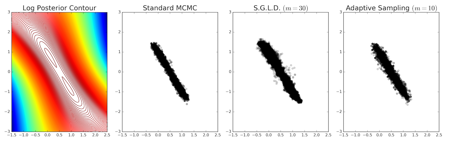
It looks like all three methods roughly obtain the same posterior form.