On Risk and the Bias-Variance Tradeoff (From Keener 3.1)

I am currently reading the textbook Theoretical Statistics by Robert W. Keener, and I thought I would write up some notes on Chapter 3, Section 1 of the book. Chapter 3 is titled “Risk, Sufficiency, Completeness, and Ancillarity,” with 3.1 specifically being about the notion of risk.

So what is risk? To understand this, we need to describe the problem setting. The goal in statistical inference is about learning a parameter vector \(\theta\) from data, where in general the data \(X\) consists of \(n\) points \(X_1, \ldots, X_n\) with \(X_i \in \mathbb{R}^k\) for some dimension \(k\).

A statistic of the data is a function of the data which provides some information about it. Keener denotes data statistics as \(\delta(X)\). Probably the canonical example of a statistic is the mean of the data, or \(\delta(X) = (X_1 + \cdots + X_n)/n\). It is worth pointing out that this only works if the \(X_i\) are random vectors, and in addition, that the mean function is many-to-one. That is, we can have different datasets that result in the same mean. Thus, the statistic \(\delta\) here only provides partial information on the data.

Our problem setting also involves some function of the parameter, which Keener denotes as \(g(\theta)\). The goal of estimation is to find a statistic \(\delta\) such that \(\delta(X)\) is “close” to \(g(\theta)\). It may not be totally clear why we introduce \(g\), but it gives us flexibility; for instance, we might only be interested in one component of \(\theta\) so \(g(\theta) = \theta_i\). For now, I find it easiest to just think of \(g\) as the identity, so \(g(\theta) = \theta\) and we want our statistic to be close to the real parameter, but throughout this post, I will be sloppy and use \(g(\theta)\) and \(\theta\) interchangeably (in my defense, Keener does the same thing).

Let’s clarify the above with the boring example of flipping a coin that can land heads with some probability \(\theta \in [0,1]\). If we flip the coin 100 times, with each trial independent of the others, then the random variable \(X\) representing the total number of heads follows a binomial distribution. (Another way to express \(X\) is therefore \(X = X_1 + \cdots + X_{100}\) where \(X_i = 1\) if the trial resulted in heads, and 0 otherwise.) If we want to get a statistic \(\delta\) that maps the data to an estimate of \(g(\theta) = \theta\), what would be a “good” statistic? The statistic \(\delta(X) = X/100\) certainly makes sense, since it is the natural proportion of samples! But is this the “best” statistic we have?

To quantify the notion of a “best” statistic, we turn to the concept of risk, which in turn relies on the concept of a loss function \(L\). The loss function \(L(g(\theta), \delta(X))\) represents the (non-negative) penalty in estimating \(g(\theta)\) (which again, I treat as \(\theta\) here) with \(\delta(X)\). Since the data \(X\) is random, \(L(g(\theta), \delta(X))\) may sometimes be large with unlucky outcomes of \(X\), so we use expectations, which is where the risk \(R\) comes from:

Note that Keener uses \(\mathbb{E}_{\theta}\) to indicate expectations with \(\theta\), but I find that a little misleading because what is random here is really \(X\), not \(\theta\). We assume \(\theta\) is fixed … but for Bayesian risk the situation is different. Hence, the above is sometimes referred to as the Frequentist risk.

Let’s continue with the coin-flipping example from earlier. Probably the most common loss function is the squared error loss, or \(L(g(\theta), \delta(X)) = (g(\theta)-\delta(X))^2\). What, then is the risk associated with the estimator \(\delta(X) = X/100\)? We apply the definition:

Where we use \(\mathbb{E}[X] = 100 \theta\) according to the definition of the expectation of a binomial random variable. To determine \(\mathbb{E}[X^2]\) we follow the familiar technique of using the formula for the variance:

Solving for \(\mathbb{E}[X^2]\), we obtain

Now let’s consider something interesting: what if we use a different estimator, defined as \(\delta(X) = (X+3)/106\)? Intuitively, this looks to provide more “smoothing” of the \(\theta\) estimate to get it closer to \(1/2\). Let’s compute the risk, again assuming the squared loss:

How do we compare the risk of the previous two estimators? It’s not clear at first glance, so we need to plot the curves. Fortunately, Keener already did this with the following image:

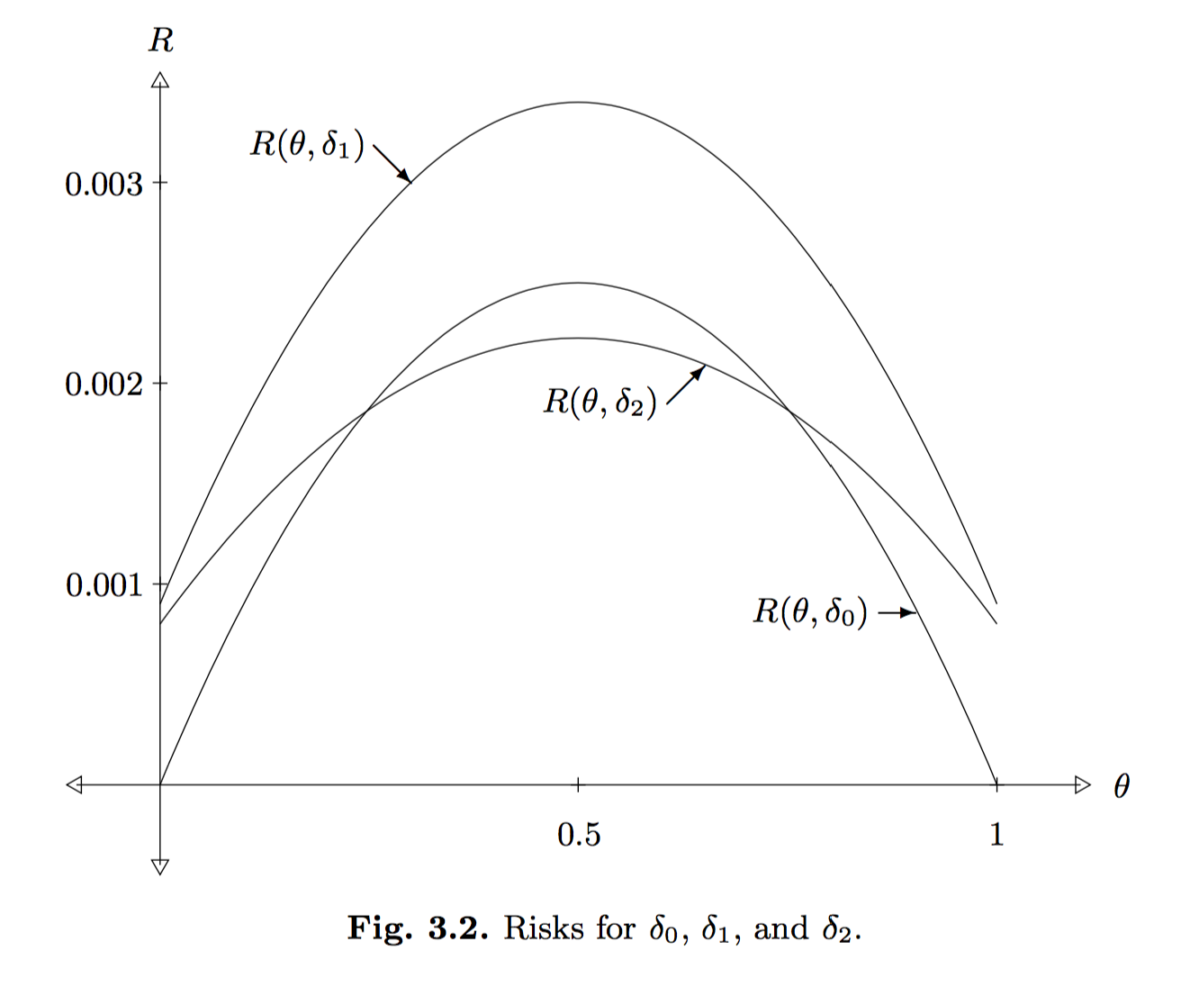
In the above, he uses a third estimator, \(\delta_1(X) = (X+3)/100\), and also, \(\delta_0(X) = X/100\) is the original estimator and \(\delta_2(X) = (X+3)/106\).

It is intuitive that \(\delta_1\) is a poor estimator of \(\theta\) because it adds 3 (i.e., like adding “three heads”) without doing anything else. In fact, we can rigorously say that \(\delta_1\) is dominated by both \(\delta_0\) and \(\delta_2\) because, throughout the entire support for \(\theta\), the risk associated with \(\delta_1\) is higher than the other estimators. The comparison between \(\delta_0\) and \(\delta_2\) is less straightforward; when the true \(\theta\) value is near \(1/2\), we’d prefer \(\delta_2\) for instance, but the reverse is true near 0 or 1.

To wrap up this discussion, I’d like to connect the concept of risk with the bias-variance tradeoff, which introduces two key concepts to know (i.e., bias and variance). The bias of an estimator \(\delta(X)\) is defined as \(b(\theta, \delta) = \mathbb{E}[\delta(X)] - \theta\), where here we write \(\theta\) instead of \(g(\theta)\) for simplicity. The variance is simply \({\rm Var}(\delta(X))\) and usually involves computations involving the variance of \(X\) directly.

Problem 1 in Chapter 3 of Keener introduces the very interesting fact that the risk of an arbitrary estimator \(\delta\) under squared error loss is \({\rm Var}(\delta(X)) + b^2(\theta, \delta)\), or more intuitively, \(V + B^2\). In fact, I earlier saw this result stated in one of the two papers I discussed in my post on minibatch MCMC methods. In Section 3 of Austerity in MCMC Land: Cutting the Metropolis-Hastings Budget, the paper states without proof:

The risk can be defined as the mean squared error in \(\hat{I}\), i.e. \(R = \mathbb{E}[(I - \hat{I})]\), where the expectation is taken over multiple simulations of the Markov chain. It is easy to show that the risk can be decomposed as \(R = B^2 + V\), where \(B\) is the bias and \(V\) is the variance.

The first thing I do when I see rules like these is to try an example. Let’s test this out with one of our earlier estimators, \(\delta_0(X) = X/100\). Note that this estimator is unbiased, which means the bias is zero, so we simply need to compute the variance:

and this precisely matches the risk from earlier!

To prove that the risk can be decomposed this way in general, we can do the following (using \(\theta\) in place of \(g(\theta)\) and \(\delta\) in place of \(\delta(X)\) to simplify notation):

as desired! In the above, we expanded the terms (also by cleverly adding zero), applied linearity of expectation, applied the fact that \(\mathbb{E}[\mathbb{E}[\delta(X)]]\) is just \(\mathbb{E}[\delta(X)]\), and also used that \(\mathbb{E}[\delta - \mathbb{E}[\delta]] = 0\).