This will probably be my last prelim review post. The topics I’ll cover in this post are convex optimization, statistical learning theory (broadly), and logic/planning. Actually, I wanted to make some detailed notes about Kalman filtering, but I think I’ve done more than enough here, and there are too many equations involved to write that quickly.

Convex Optimization

This part is based on sections 9.1 through 9.5 of Boyd and Vandenberghe’s book, freely available online. Stephen Boyd also has a lecture video on YouTube that I watched, which I found to be very helpful. (I can also understand Professor Boyd’s speech well.) The book is fine, I suppose, but is really hard for me to read so I made embarrassingly slow progress as I learned this material.

The main purpose of sections 9.1 through 9.5 is to discuss iterative algorithms for minimization. Formally, we have the problem of minimizing a convex function \(f(x)\) and need to find the optimal \(x = x^*\). As in almost all cases, we have to remember that \(x\) is not generally a scalar but a vector, but \(f\) is real-valued, so \(f : \mathbb{R}^n \to \mathbb{R}\). I had to keep reminding myself of this.

In most cases, we need to use iterative algorithms to find \(x^*\). The class of algorithms we use are known as descent algorithms because they generate points \(\{x^1,x^2,\ldots \}\) such that \(f(x^k) > f(x^{k+1})\) unless we are at the optimum. Actually, a little side-note: there is exactly one optimal \(x^*\) because we are actually assuming that \(f\) is strongly convex, not just convex (and strong convexity is not the same as strict convexity!). By strong convexity, we assume that there is a constant \(m > 0\) such that \(\nabla^2 f(x) \ge mI\), which means \(\nabla^2 f(x) - mI\) is positive semidefinite.

A lot of our future analysis will depend on a concept known as the condition number of a matrix or a set. For a matrix, the condition number is the ratio of the largest singular value to the smallest singular value. Alternatively, we can use eigenvalues if the matrix is positive semidefinite, which actually happens here since the second-order characterization of convexity states that the Hessian of \(f\) is positive semidefinite. The condition number of a set is defined as the ratio of the largest width to smallest width. High condition numbers result in highly skewed/stretched data.

Here’s the descent algorithm. We repeat the following until some stopping criterion:

• Compute a (descent) direction to change \(x\), denoted \(\Delta x\)
• Compute a length or step size \(t\) to go in that direction using some form of line search
• Compute \(x \leftarrow x + t (\Delta x)\)

There are two main ways to choose \(t\): exact search (find \(\arg_t \min f(x + t (\Delta x))\)) or backtracking search. For some reason, it took me a really long time to understand backtracking line search, but after looking at that figure in Boyd’s book for ages, I understand what it does now. We have to keep decrementing \(t\) until our function \(f(x + t (\Delta x))\) lies below a given upper bound. Backtracking line search is important because it’s more efficient and in practice, it often works just as well (or better!) than exact line search. To explain it, remember that figure with the three curves in it: one is \(f\) and two are straight curves which follow from the FOC of \(f\) at \(y=x+\Delta x\).

But the real difference in the various gradient algorithms comes when we pick \(\Delta x\). There are three options:

• Use \(-\nabla f(x)\). I mean, the gradient \(\nabla f(x)\) points in the direction of greatest increase of \(f\) at \(x\) (by definition) so why on earth would we not use the negative of that? This is gradient descent.
• Use the direction that maximizes the negative gradient in the direction determined by a pre-specified norm. Precisely, our first-order approximation of \(x\) at \(x-v\) is \(f(x+v) \approx f(x) + \nabla f(x)^Tv\), and we want to find \(\arg_v \min \{\nabla f(x)^Tv : \|v\| \le 1\}\); in other words, we want to make the directional derivative as negative as possible. We need to restrict \(\|v\|\) because if not we could first pick a direction that makes it negative when multiplied by the gradient, and then make it arbitrarily large. Also notice that we are not specifying the exact norm. This is steepest descent, and equals gradient descent when \(\|v\|\) is the \(\ell_2\) norm.
• use \(-(\nabla^2 f(x))^{-1}\nabla f(x)\), i.e., the negative of the inverse of the Hessian, multiplied by the gradient. Whew! This comes from the second order approximation of \(f(x + \Delta x)\) – just take the gradient with respect to \(x\), then solve. This is Newton’s Method.

Gradient descent is simple, and works perfectly (i.e., converges in one step) when the data are “isotropic,” that is to say, roughly “equal in all directions.” It’s bad when the condition number of the Hessian or the sublevel sets is high (e.g., in the 1000s). The classic example is the ellipsoid “bowl” where we have a 3-D bowl that is much wider in one direction than the other. Gradient descent with exact line search will always “overshoot” the optimal location and keeps going back and forth, zig-zagging to the center. The stopping criterion for gradient descent is if \(\|\nabla f(x)\|_2 \le \eta\) for some pre-specified \(\eta\).

Steepest descent is a generalization of gradient descent in that we get the option of picking the norm that we want to use as a metric of our “gradient” here. A quick warning: there are actually two versions of \(\Delta x\). I tend to assume we are using the normalized version \(\Delta x_{\rm nsd}\), where the \(v\) we pick has norm bounded by one. There’s also the un-normalized version \(\Delta x_{\rm sd} = \|\nabla f(x)\|_{*} \Delta x_{\rm nsd}\) but I don’t understand how this actually works.

Steepest descent can work with the \(\ell_1\), \(\ell_2\), and quadratic norms. In the \(\ell_1\), it is equivalent to coordinate descent (modifying one coordinate of \(x\) at a time), and the way to think about this is that we are taking the maximum component (in absolute value) of \(\nabla f(x)\) and setting our \(v\) to be zero everywhere except for \(\pm 1\) at that “largest component.” The derivation for \(\Delta x_{\rm nsd}\) in the quadratic norm is more complicated (for the un-normalized, it’s just \(-P^{-1}\nabla f(x)\)), but visualizing it is easier: we have a point \(x\), draw an ellipse around it (determined by the norm), and then pick the direction that results in the greatest decrease. More intuition: extend as far as possible in the direction of \(-\nabla f(x)\), while staying inside that unit ball. It’s also worth noting that we can transform coordinates from the quadratic norm’s matrix \(P\) to get gradient descent. In fact, this gives a useful test for a norm: how well steepest descent performs will depend on how well the transformed points \(P^{1/2}x\) have “equal” isocontours suited for gradient descent.

Newton’s method is a step up from gradient descent in that we use a second-order approximation of \(f\). The way I think of it is that gradient descent will produce a plane in 3-D (e.g., for a 3-D “bowl” that we’re trying to reach the minimum of) but Newton’s method will produce another bowl, though this bowl will usually be entirely above of the original one, save for the tangent point.

The book mentions three “perspectives” on Newton’s method:

• Minimization of the second-order approximation of \(f\), which is how I see it.
• Steepest descent in the Hessian norm: it’s like the quadratic norm described earlier, but the Hessian is a really good “\(P\)” matrix to use since its condition number approximates the condition number of the sublevel sets!
• Solution of linearized optimality condition. I did not understand this at first, but actually, think of Newton’s method for approximating roots of a function \(f\), where we need to subtract \(f/f'\). In our case, we want to find the minimizer of \(f\), which means we want the roots of the derivative \(f'\), which involves \(f'/f''\). That’s exactly what we have here!

More facts about Newton’s method:

• If the original function is already quadratic, Newton’s method converges in one step.
• It is independent of affine coordinate transformations. When we do iterates with \(x^{(k)}\) versus \(Tx^{(k)}\), the relationship between the points will remain the same.
• It uses something called the Newton decrement \(\lambda(x) \approx f(x) - f(x^\star)\) to determine when to stop.
• There is a damped phase versus a pure phase. In the former, the difference in \(f\) when we change \(x\) decreases by a fixed quantity (this is good!). In the latter, the backtracking line search always picks \(t=1\) and the number of accurate digits doubles. Thus, there is no need to run that second phase more than, say, four times.
• Newton’s method still works with badly-conditioned sublevel sets of \(f\).
• The downside of Newton’s method compared to gradient or steepest descent is that (1) we have to compute the Hessian, and (2) we have to store it – remember that the Hessian will be \(n \times n\), whereas the gradient will only be \(n \times 1\).

The usual disclaimers apply in that we don’t really know various constants that get involved in the proofs, unfortunately.

Statistical Concepts and Logistic Regression

This part is closely related to what I wrote about linear regression and the least mean squares algorithm. I will be discussing logistic regression as well (for classification, not regression), but first we take a brief detour to discuss the third major class of problem known as density estimation.

The problem is, given data, to find the appropriate model for it. The relatively easy case is if we assume we already have an idea of the distribution (e.g., Gaussian) and we just need to find the parameters (here, the mean and variance). We find the parameters via maximum likelihood. So in the IID Gaussian case, of which the graphical model is represented as \(N\) independent shaded circles in a graphical model, we take the sample mean and sample covariance as our MLEs. With the Bayesian approach, where we have a new \(\mu\) node pointing to all samples, we put a Gaussian prior on mean \(\mu\) so that the result is a weighted estimate (and the same for the variance, actually), because of conjugate priors. In the case of discrete data \(x\), we model these with multinomials. The resulting MLEs, which require Lagrange multipliers to solve (which gave me a huge headache at first), are just the sample proportions. For the Bayesian version, we use a Dirichlet prior. To extend the class of distributions we want to model, we can assume a mixture model, where \(p(x\mid \theta) = \sum_{i=1}^{k}\alpha_i f_i(x\mid \theta_i)\), where the \(\alpha_i\)s are mixing proportions that sum to one. This time, we have a hidden node that points to its own observed data point \(x\).

There is an alternative strategy of estimation known as nonparametric density estimation. Here, we do not assume we have a fixed parameter \(\theta\) and as our data grows, the nonparametric model will grow to represent a wider class of distributions. We have kernels, where each data point takes some probability mass, and we add them up and normalize. In the case of Gaussian kernels, the nonparametric case for a fixed number of samples really reduces to the mixture model case, but they differ as the number of instances grow.

Tip: use the nonparametric case if we do not have a good idea of the model and lots of data, but use the parametric version when we have little data and a good idea of its underlying distribution (it will converge faster). The line between the two methods does blur somewhat, for instance, when we have a mixture modeling problem where we have to dynamically estimate the number of components \(K\).

Finally, we can turn our attention towards the regression and classification problems. In both cases, we model \(p(y_n\mid x_n,\theta)\), where the \(n\) here indicates that we assume IID data. For linear regression, we assume \(y_n = \beta^Tx_n + \epsilon_n\), and have to find \(\beta\). The choice of \(\epsilon_n\) is what really determines the distribution – here we assume Gaussians, so this is linear regression, and that means the MLE of \(\beta\) is the OLS estimate. Another way of extending linear regression to be more flexible is to use (conditional) mixtures. Here, the graphical model looks like that of the density estimation mixture model, except we also need the \(X_n\) node (which may or may not be connected to the mixture node \(Z_n\)). And, of course, we could always treat these from a Bayesian perspective, perhaps by endowing that \(\epsilon_n\) error term for Gaussians (in linear regression) with Gaussian priors for its mean and variance (well, probably variance only if we want the mean to be zero).

We can also use nonparametric regression, if we do not want to restrict our conditional mean functions. Actually, Russell and Norvig cover this a bit in their nonparametric methods section in the textbook; each predicted new \(y\) is based on the weighted prediction of the other, “nearest” \(y_n\)s.

In the classification case, the distinction between generative and discriminative cases is more apparent. I remember the way the arrows point in the model just by remembering the discriminative case, and then realizing that the generative is the opposite one. Use the generative case if we want a full probabilistic model, and use discriminative classification if we only care about the boundary point. The full model in the generative case also may help combat overfitting, so it is better with limited and partially observed data. Discriminative models have less bias because they make fewer assumptions, so they work better with lots of data (in fact, it’s a lot like how nearest neighbor will work best with lots of data).

These approaches are important to understand the logistic regression algorithm, where we assume that the posterior probability \(p(y=0\mid x, \theta)\) for a binary classification problem is logistic or arrives at that form. That we have the inner product there means the posterior “boundaries” of equal probability are hyperplanes. In the generative case, we estimate means and covariances, which define \(\theta\) (and these are density estimation problems!) and the boundary implicitly, while in the discriminative case, we estimate \(\theta\) “directly,” possibly choosing an arbitrarily complex boundary. In fact, “discriminative = logistic regression”, “generative = Naive Bayes”, and both are for classification. In fact, that’s why they are in the same chapter of Mike Jordan’s notes!

Again, logistic regression assumes we have the sigmoid function as the form for our posterior probability. We can assume this from the outset (discriminative) but we can also “inspire” this generatively. Here’s how: assume that we have two classes, and the class conditionals¹ are Gaussian with, and this is important, the same covariance matrices. Then the posterior \(P(Y = 0 \mid X, \theta)\) can be expressed as \((1+e^{-\beta^Tx - \gamma})^{-1}\), i.e., the exponent has an affine function of \(x\), which means that the boundaries of equal probability are hyperplanes. In the special case of equal mixing proportions, we have equidistant boundaries. A skewed mixing proportion will shift the boundaries towards or away one of the classes.

In fact, the assumption of a Gaussian class conditional is not even necessary. We can get away with multinomials (this is another way of viewing the Naive Bayes classifier), or in fact, anything in the exponential family²! When I was learning about these in my undergraduate Bayesian statistics course, I never really got why the exponential families were that important. But here is one reason, I suppose. Note that these are still assumptions that add bias to the generative case.

We can extend the previous analysis to the general classification case with \(K\) outputs. In that case, we use the softmax: \(e^{\beta_i^Tx}/\sum_j e^{\beta_j^Tx}\), which also results in linear boundaries, though that’s kind of stretching the definition; imagine a “pie-chart” where the “slices” represent boundaries. Also, if we wanted to find maximum likelihood estimation, we could do that, because we have \(P(x\mid y,\theta)\) and \(P(y\mid \theta)\). Just combine those to get the joint and differentiate the log of it. For instance, in the two Gaussian case, the MLE for the means \(\mu_1\) and \(\mu_2\) are just the sample means of the elements in their respective classes (remember, we assume we know the training data labels), and the covariance is weighted among the two. In the general case, we again write the formula and then separate the terms appropriately. Note: we will use \(\theta\) to represent a generic vector of weights. To be safe, whenever we write probabilities, add a conditioned \(\theta\).

Whew! Now we can talk about logistic regression, where the class dependency is fixed to be a sigmoid function. How do we find the best \(\theta\)? As usual, take logs, and maximize. This actually leads us to an LMS-like algorithm, and the only difference is the class expectation. For the batch version, we use iteratively reweighted least squares, which is basically Newton’s method for optimizing the (nearly) quadratic log likelihood function. In fact, there is a close connection between this method and the “normal” weighted least squares method, which started by assuming that each training input/output had an attached “weight” to it: this method can be written as

\[\theta \leftarrow (X^TWX)^{-1}X^TWz\]

for what I thought was a pretty convoluted \(z\), but actually turns out to be a first order approximation of \(y\). Interesting … I don’t really understand the full details of this, but having the knowledge of convex optimization at the top of this post really helped me.

For extending discriminative learning to multiple classes, again assume that \(P(Y = ? \mid X,\theta)\) is represented by the softmax function, and a lot of our math follows for what is known as softmax regression.

Finally, thanks to Andrew Ng I have a bit of a better idea on the connection between the logistic regression update (in the LMS-like form) versus the perceptron: just change the sigmoid part in the update to be the “sign” function, and then the update turns into the perceptron.

More Statistical Learning Theory

Here’s a random assortment of notes from Mike Jordan’s book (which I think he has abandoned now).

First, let’s consider the multivariate Gaussian is one of the most important distributions to understand, and I did not have an easy time learning about it. Fortunately, by now I can write out the formula and reason about it quite easily. Unfortunately, I don’t know how to derive it from first principles. I can explain “roughly” what it does, e.g., that \(|\Sigma|^{1/2}\) in the normalizing constant comes from how each component of the random vector contributes some amount of variance equal to its eigenvalue, and the determinant of a matrix is the product of its eigenvalues.

But anyway, there are a few important facts worth discussing about the multivariate Gaussian.

• There is a moment parameterization and the canonical parameterization. The former is what I always use, but we can transform it into the latter with the rules \(\Lambda = \Sigma^{-1}\) and \(\eta = \Sigma^{-1}\mu\) to get \(p(X\mid \eta, \Lambda)\).

• Given a matrix \(M\) where we partition it into components \(E,F,G,\) and \(H\), the goal of block diagonalization is to find matrices \(A\) and \(B\) such that \(A \times M \times B\) is diagonal in the corresponding locations of \(F\) and \(G\). After a lot of algebra, we can arrive at the derivative of the partitioned matrix \(M\), and also derive a bunch of useful identities (the “matrix inversion lemma”) that I refuse to memorize.

• The reason why we go through this tedious algebra is that it gives us identities we can use when partitioning the multivariate Gaussian to get formulas for marginal and conditional probabilities involving multivariate Gaussians. Specifically, we have \(x\in \mathbb{R}^n\) split into \(x_1\) and \(x_2\), and we want \(p(x_2)\) and \(p(x_1\mid x_2)\), where I’m eliding the parameters for simplicity. We obviously have the joint \(p(x_1,x_2)\), so we need to figure out how to split them cleverly. Once we’ve gone through the derivation, we will find that the moment parameterization lends to easy computations of marginals but hard ones for conditionals, and the reverse is true for the canonical parameterization. Importantly, these formulas preserve the fact that our variables are Gaussian.

In addition to knowing that the marginals and the conditionals are Gaussian, the sum of independent Gaussians is Gaussians.

We can extend the mixture model discussion from last section into the multivariate Gaussian setting, where the hidden variables indicate the particular multivariate Gaussian distribution of interest. Here, we have \(p(x\mid \theta) = \sum_i \pi_i \mathcal{N}(x\mid \mu_i, \Sigma_i)\), and assuming IID points, we want to find the \(\pi\), \(\mu\), and \(\Sigma\) parameters to maximize the log likelihood. This requires Expectation-Maximization, which involves computing the probability that a particular distribution generated point \(x\), which is of obvious interest for classification. (Admittedly this case works best in the binary setting where the conditional expectation is the same as the conditional probability of being one.) One can also think of K-Means as a simplified version of EM. We use EM rather than maximum likelihood because our “log” term has a sum inside it, which is due to the probabilities of the point being in multiple possible classes. In the previous section (on classification), we had the class so we effectively take only one term in that summation, in which MLE follows easily.

One thing I didn’t quite realize earlier was that in the EM for Gaussians, we can take the log likelihood, differentiate it with respect to \(\pi_i\) (or \(\mu_i\) or \(\Sigma_i\)) and we end up finding solutions that match the EM algorithm, which is interesting and implies that our “heuristic” update formulas may not be so bad because they indicate maxima of the log likelihood. Of course, one can also derive the update formulas “systematically” by appealing to the expected complete log likelihood, where we take expectations with respect to the hidden variables. (See my previous post for more information about this quantity.)

The E-step in general involves computing the expected complete log likelihood, and the M-step in general involves maximizing the expected complete log likelihood with respect to \(\theta\). The full power of this terminology is not needed in the simple Gaussian example, but it is a useful exercise to ensure that we derive the same update formulas we developed “heuristically.” In general, the expected complete log likelihood does not suffer from the “coupling” of variables as the original log likelihood.

Finally, we consider the “mixture of experts” case, which is when we have a mixture model for the purposes of regression or classification. Mike Jordan’s notes appear to be missing some figures, so it’s a little hard to see what he’s trying to do, but I think the first figure represents a “V”-shaped set of data, and we need to fit two different regressions on that. The key is figuring out where to split, which is our “EM-like” task. In the mixture of experts, the M-step involves two different maximization steps.

Logic and Planning

I discussed this earlier and had a chance to re-read all of that stuff. My main purpose in this section is to highlight how everything in this section connects with each other. I don’t want to just learn propositional logic, then first order logic, etc., I want to describe then in terms of each other, and to discuss all the similarities and differences among them (and the algorithms they inspire). But this won’t be long because Stuart Russell isn’t on the prelim committee this time (hint hint…).

But first, a laundry list of facts that really confused me the first time:

• Propositions consist of literals, which are just like the atomic elements of propositions, but they can have a “negation” symbol. That’s it: think of literals as either \(A\) or \(\neg A\).
• Predicates are really functions that output a True or a False. Predicates are – in my opinion – the backbone of first order logic.
• Be sure to realize that \(\alpha \Rightarrow \beta\) is the same thing as \(\neg \alpha \vee \beta\). This is probably the most important thing to remember to understand Horn and definite clauses, and why we can apply Modus Ponens to them.

Now we can talk about the connections. Here they are:

• One can convert from first order logic to propositional logic by extending universal and existential quantifiers.

• Forward and backward chaining play a role in both propositional and first order logic. They are algorithms for determining entailment when we assume that our knowledge base consists of Horn clauses (prop.) or first order definite clauses (FOL). This is a simplifying assumption, but it is often easy to convert databases to this format. The reason why Horn or definite clauses are needed is that their truth values are equivalent to \(\alpha \Rightarrow \beta\) (and we need “or”s not “and”s), and that exactly fits the description of the Modus Ponens and Generalized Modus Ponens rule format. Note: we use these when we do not want to use the full power of resolution.

• As an alternative, say we do not have definite clauses and are just looking for a satisfying assignment to a disjunction of clauses. Then in both types of logics, we have the option of backtracking and local search. Both of these have their similarities in the Constraint Satisfaction Problem domain. In backtracking search, we have similar versions of “minimum remaining values” and “least constraining value” heuristics. In local search, that is when we are starting with a full, though not typically satisfactory, assignment to a problem in CNF form, and we pick clauses to shift, and this is the same as in CSPs when we start with a full assignment and use the minimum conflicts heuristics to adjust values.

• The PDDL language (Chapter 10) is about a simplified language that uses first-order logic “materials” (e.g., predicates, quantifiers, etc.) to encode a search problem (remember Chapter 3!)³. Since we’re encoding a search problem, we need to define the actions we can take, and those must have preconditions and effects, which involve adding or removing some fluents. The fluent, by the way, is the atomic set whose values represent a state. Again, the really important thing to know about Chapter 10 is that it is really another case of the general search problems. One can also make plans using a logical agent.

• Knowledge representation (Chapter 12) is all about encoding “real-world” stuff in first order logic. Our strategy to represent these is formally called ontological engineering. They discuss categorizing objects, categories (make them into objects!), and events.

• Let’s go over the different kinds of algorithms:

  • Backtracking search: when we incrementally look for assignments to stuff, and then “backtrack” when we have seen some “problems”, e.g., impossible situations (and this can be used for entailment as well!). There are heuristics for this. We do this in CSPs and searching for satisfying assignments in propositional logic. We can also transform a classical planning case to a propositional case and turn it over to the backtracking solver, but this is not practical.
  • Local search: we start with a complete assignment, and move variables around until we get to a solution. We do this with CSPs, propositional logic.
  • Forward chaining and backward chaining are algorithms for deciding entailment in the two logics. We do not use these in CSPs or classical planning. The FOL case is more complicated due to the need to perform unification (among other factors), but we have general heuristics for improving them.
  • In PDDLs, we do forward searching and backward searching to search for a satisfying sequence of actions. The forward searching part is similar to the backtracking search in that we can search for actions with heuristics and backtrack if needed. Backward search can avoid irrelevant states, though.

---

Here is a random assortment of notes I created to wrap up some of the remaining material I need to know. It’s “part 1” because I have another part coming up later.

Information Theory

This part, Chapter 2 from Cover and Thomas, is a bunch of definitions and straightforward theorems (i.e., those that follow directly from definitions):

• Entropy: \(E(X) = -\sum_{x} p(x)\log_2 p(x) = -\mathbb{E}[\log_2 p(X)]\), where \(x\) is a realization of variable \(X\). It’s the amount of uncertainty inherent in a random variable. For a fixed variable \(X\) with some probability distribution that we can create, the entropy is highest if we make the distribution relatively uniform, and lowest if we make it “peaked.” In the extreme case, if we set \(Pr(X = 0) = 1\), then \(E(X) = 0\).

• Mutual Information: \(I(X;Y) = E(X) - E(X|Y)\). It’s the decrease in entropy (upon obtaining the value of \(Y\)), for variable \(X\). Note that \(I(X;X) = E(X)\) since the second term will be zero. Alternatively, we represent it as

  \[I(X;Y) = \sum_x \sum_y p(x,y) \log_2 \left(\frac{p(x,y)}{p(x)p(y)}\right)\]

  Note that \(I(X;Y) = I(Y;X)\), so it does commute.

• Relative Entropy (KL-divergence): \(D(p || q) = \sum_{x} p(x)\ln \left( \frac{p(x)}{q(x)} \right)\). This is a non-symmetric measure of the difference between distributions \(p\) and \(q\). We can also interpret it as the number of additional bits we will need to represent \(p\) if we are using the (inferior) approximation of \(q\). It is infinity if there exists an \(x\) such that \(p(x) > 0\) but \(q(x) = 0\).

All three of the above quantities are non-negative.

Another concept that plays a huge role in information theory is the following:

• Jensen’s inequality: for a convex function \(f\), \(f(\mathbb{E}[X]) \le \mathbb{E}[f(X)]\). For a concave function, like the logarithm, we flip the sign (actually for logs, we can drop the equality case). I find it easiest to remember this rule by expanding out the equations for binary random variables. Let’s say they taken on values 0 and 1 with probability a half each. Then we have \(f(\mathbb{E}[X]) = f(.5 \times 0 + .5 \times 1)\) and \(\mathbb{E}[f(X)] = .5 \times f(0) + .5 \times f(1)\) and can directly relate this to the definition of convexity.

Based on the previous discussion, we can define and infer things like:

• Joint entropy \(H(X,Y) = - \sum_x \sum_y p(x,y) \log_2 p(x,y) = H(X) + H(Y\mid X)\).

• Conditional entropy, conditional KL divergence, conditional mutual information. For the sake of simplicity, I will not write all the rules here, but here is the one for conditional entropy: \(H(Y\mid X) = -\sum_x p(x) H(Y \mid X=x) = -\mathbb{E}_p [\log_2 p(Y\mid X)]\). Note that \(H(Y\mid X) \ne H(X\mid Y)\).

• The chain rule for entropy, relative entropy, and mutual information. Unlike normal probability, these sum the components rather than multiply, which makes sense because all three cases involve logarithms. Again, I won’t write all the rules here, but will note that entropy is the easiest to relate to probability because we literally copy formulas from probability, but use sums instead of products. For the chain rule with mutual information, just pretend we don’t have \(Y\) and follow the probability convention (but sum up). Then stick the \(Y\)’s after the semicolon, but before the conditioning bar. For KL-divergence, it’s the same (split up the joint into a marginal and product, but do this for both distributions, then use two “D” terms.

• A theorem: \(H(X) \le \log_2|\mathcal{X}|\), where \(\mathcal{X}\) represents the range of variable \(X\), and equality here holds if and only if \(X\) is a uniform random variable.

• Also one thing that tricked me up the first time I saw it was this consequence of Jensen’s inequality:

  \[\sum_{x \in A} p(x) \log\left( \frac{q(x)}{p(x)}\right) \le \log \left( \sum_{x \in A} p(x) \frac{q(x)}{p(x)} \right)\]

  where \(A\) is the domain for \(p\). I am assuming this really means

  \[\mathbb{E}_p\left[\log \left(\frac{q(x)}{p(x)}\right)\right] \le \log \left( \mathbb{E}_p\left[ \frac{q(x)}{p(x)} \right] \right)\]

A final thought on this section: an alternative interpretation of entropy is that it is a lower bound on the average number of bits required to represent the random variable. It’s not “the minimum number of bits” because random variables take on different values with different probabilities, so we may wish to allocate more bits for the low probability events. And we also need to make it clear how we encode, so that we can compare different encodings. Example 1.1.2 from Cover and Thomas will clarify: here, we have eight horses, and they each win with some specified probability. If we wanted to encode the random variable \(H\) indicating the horse that won, we could use three bits in the standard way. But this is suboptimal if the distribution is \((1/2,1/4,1/8,1/16,1/64,1/64,1/64,1/64)\), like it is in the example, because we should allocate fewer digits to the higher probability horses, and more towards the ones that are less likely to win. It’s possible to encode \(H\) so that the average number of bits to represent it is two, which exactly matches the entropy.

Decision Trees

Decision trees are one of the simplest nontrivial classifiers¹ that have strong performance in practical tasks. The hypothesis space is the set of trees. For each \(n\)-dimensional sample \(x\), we classify it by propagating \(x\) down the tree. At each node, we test an attribute \(x_i\), and depending on that value, send the sample left or right. Once we send it down the tree far enough, it will land in some “classifier” node that labels the class of that element.

Great, so how do we train such trees from labeled data \(\{(x^{(i)} = (x_1,x_2,\ldots,x_n)^{(i)},y^{(i)})\}_{i=1}^n\)? For that, we invoke some information theory criteria: we want to select the attribute to test that will result in the most amount of purity in the resulting trees, where purity is defined based on entropy. Formally, at each point of the tree, we have a set of data and a candidate set of attributes. We pick the attribute that maximizes the information gain of the data.

Let’s precisely define this for boolean decision trees. At a decision tree’s node, we have \(p\) positive and \(n\) negative samples. The entropy of the random variable describing the output is the entropy of a binary random variable with probability \(p/(p+n)\); to simplify the subsequent notation, denote this as \(B(p/(p+n))\). We define the gain of attribute \(A_k\) that splits the data into \(d\) subsets as follows:

\[Gain(A_k) = B\left(\frac{p}{p+n}\right) - \sum_{i=1}^d \left( \frac{p_k+n_k}{p+n}\right) B\left(\frac{p_k+n_k}{p+n}\right)\]

For each subset, we weigh its entropy probabilistically. Otherwise, you could think of a useless attribute that keeps the same proportion of positive and negative examples in each subset. Without the probability weighting, splitting on \(A_k\) would increase the entropy of the goal test on the data.

There are other impurity measures, such as the Gini impurity measure \(\sum_{k=1}^K p(x_k)(1-p(x_k))\) if the output takes on \(K\) realizations. This is not the same as the measure of income inequality! I think the “CART” category of decision trees uses the Gini measure, whereas the “C4.5” and “C5” trees use entropy to measure impurity, though I think the boundaries between those categories is a bit blurry. Misclassification error is not an appropriate measure because it – unlike Gini impurity and entropy – does not give higher weight to branches with purer solutions.

Here are some things to think about:

• Trees can overfit, so what happens in most realistic algorithms is that we build the large tree first, then prune away nodes with only leaf descendants that do not contribute much to the information gain (e.g., using tests of statistical significance to see if the gain is significant enough). This is not the same as building a tree and deciding to prune away early. The classic example is the XOR data. If we have a lot of XOR data that we want to split, we will find that the information gain of both attributes is zero. We do not want to prune away early because the next step will involve splitting on the second part of the XOR, which splits the data perfectly.

• In practice, information gain might not be a good value of the amount of information in an attribute, because there might be an attribute that maps each element to a unique value.

• We may have missing data. A simple but bad strategy is to ignore all training data points that have missing data. An alternative is to “fill in” those values probabilistically based on the distribution of values of those variables in the other samples considered for a particular decision tree.

• We may want to use decision trees for regression if the output is continuous-valued. One option is to use a decision tree normally up to a certain depth, and then after that, we fit (linear) regression on only those data points that manage to reach that particular leaf node, and only the subset of variable attributes yet to be tested.

  How would we train such a regression tree? HTF suggest a greedy algorithm (which also assumes continuous attributes, by the way): at each node, find the attribute and a split point that minimizes the sum of squared errors of the two resulting regions. HTF also assume that once we get to a region, we will approximate the samples with just one value, rather than doing a full-blown regression on it, which makes the problem a lot easier since the sum of squared errors criterion means we pick the mean of the elements considered at that node. To avoid overfitting, they suggest weakest link pruning. We iteratively pick the internal (non-leaf) node that, upon its removal (and subsequent collapsing of the tree) results in the smallest increase in the sum of squared errors criterion. This is pretty cool, and it’ similar to what Russell and Norvig describe.

Finally, here’s a rather interesting connection between boolean decision trees and propositional logic that I failed to realize at first: we can label various paths throughout the tree as \(Path_i\), and so the goal is expressed as:

\[Goal \iff (Path_1 \vee Path_2 \vee \cdots )\]

Thus, any function in propositional logic can be expressed as a decision tree!

Nearest Neighbor

This classifier is easy to describe: for each test point, we look at the \(k\) nearest points according to Euclidean (or other) distance matrices and classify the test point as the majority class among those \(k\). This is a problem in high dimensions, since the notion of “distance” as a measure of similarity becomes less reliable due to a combination of (1) noisy and irrelevant features, and (2) the rather intriguing fact that the higher we go in dimensions, the more likely it is our points are farther away from each other. As we increase the dimension of the unit hypercube with our fixed \(k\)-nearest neighbor classifier, we will need to traverse an extra amount for each dimension to reach the \(k\) nearest neighbors.

Let’s now restrict our focus to the 1-nearest-neighbor case. On the surface, this might seem to be unreliable, since we’re only using one closest point and it might overfit the data (see examples of plots showing 1-nearest neighbor versus 5-nearest neighbor). But a famous result called the Cover-Hart Theorem provides a different story, saying that the asymptotic error rate of the 1-nearest neighbor classifier is never more than twice the error of the Bayes’ classifier (according to HTE), where the Bayes’ classifier assigns \(\arg_y \max P(y\mid X=x)\). While it sounds nice, it assumes that new points have to exactly coincide with a point in the training data, which is true in the limit, but not true in general.

Here’s another interesting fact about nearest neighbors that I found surprising. Researchers used nearest neighbors to achieve the best performance (at that time) on the MNIST handwritten digit recognition problem. The digits themselves are points in \(\mathbb{R}^{256}\)-space. A classifier would have to work in high dimensional space and be invariant to rotations, scaling, etc. They way they did this was by defining manifolds in \(\mathbb{R}^{256}\)-space. For instance, there is a one-dimensional curve where points on that curve represent different rotated versions of the “3” digit². Then there can be another curve representing a different three. One idea is to take the Euclidean distance of the two closest points \(p_1\) and \(p_2\) which lie on separate curves. Unfortunately, this may result in heavily rotated images being equivalent (the classic disaster: confusing a “6” with a “9”), so the ingenious solution is to use tangent lines. That’s the intuition: in reality, the “one-dimensional curves” would be manifolds taking into account additional invariance factors.

Having motivated nearest neighbors, let’s discuss some of its drawbacks. One problem is that it needs to store all the training instances, and for each new test point to classify, it needs to iterate through all of those to find the \(k\) closest neighbors. If \(O(n^2)\) time is unacceptable, then we can speed up the process of finding nearest neighbors with the following two strategies:

• We can use \(k\)-d trees, or more accurately, \(n\)-d trees if our data is \(n\)-dimensional, so that we don’t confuse this with the \(k\) in the \(k\)-nearest neighbors. At each node, this tree will pick a dimension \(i\) and split the examples according to their median point so that all \(x_i\) such that \(x_i < m\) will go the left sub-tree, and the rest go to the right subtree. The dimensions are typically chosen based on the widest spread of values.

  Thus, if we are doing 1-nearest neighbor, for a given new point \(x\), we find its nearest neighbor by querying the \(k\)-d tree to see where it would be located (i.e., it’s like we are inserting it in the tree). We proceed until we hit a leaf, and declare that as the best node found given the current information. But we have to be careful. The nearest neighbor of \(x\) might not be in the same hyperplane after a split! We need to “backtrack” and then measure the distance between \(x\) and the hyperplanes at each step, to see if there are nearest neighbor candidates on the other side. Check the Wikipedia page for more details. They have a nice description and an animation.

  The downside with \(k\)-d trees is that with many dimensions, we will need to keep track of numerous subtrees that could potentially have “that nearest neighbor,” and we would iterate through the entire tree. To extend this algorithm for multiple neighbors, we use a list of nearest neighbor points.

• We can use locality sensitive hashing, which hashes “similar” values in high dimensional spaces to the same hash buckets. Then, using only the elements remaining in that bucket, we can perform exact nearest neighbor via brute force comparisons. Since hash functions are hard to create, we can try \(M\) hash functions independently to get \(M\) buckets, then take the union of all those elements to arrive at the set which we will use for exact comparisons. Russell and Norvig seem to suggest that each of those \(M\) hash functions be a projection down to a line, and the buckets would be a line segment. I guess that makes sense.

  The downside with locality sensitive hashing is that it, unlike the use of \(k\)-d trees, is an approximate nearest neighbors search.

Nearest neighbors has an interesting tradeoff with perceptrons. Kernelized perceptrons learn similar to the way nearest neighbors learn, especially with Gaussian kernels that weigh a probability distribution about each point. In other words, distance-weighted nearest neighbors are kernelized perceptrons. Nearest neighbors, unlike plain (non-kernelized) perceptrons, can use fancy similarity functions, as exemplified by the handwritten digit recognition example.

HTE also emphasize the connection between nearest neighbors and least squares.

(Artificial) Neural Networks

Neural networks are a natural extension of the perceptron that I’ve written about in detail before, since perceptrons form the basic building blocks for each node. Like the perceptron (and regression, for that matter), we develop a classifier by updating weights. For neural networks, we use backpropagation to update the weights. At a high level, this means for each training instance, we “feed” it to the network so that it classifies it. Then, we propagate the “error” backwards through the network to update weights. The weight update for those connecting to the output layer is the same for that of logistic regression³, assuming we’re using the sigmoid nonlinear function. The real challenge comes when we compute weight updates for those connecting input or hidden layers to other hidden layers. But in fact, the gradient for the loss at inner nodes is the same as the computation for the gradient at the output layer, except we apply the chain rule multiple times. I’m not going to write the derivation here since it would take too much time; I just did it by hand.

Neural networks have an intriguing fact: provided that there are sufficiently many nodes and layers, they can represent any continuous function (of the input) with arbitrarily high accuracy. It needs multiple layers with non-linear activation functions at each node. Otherwise, if a NN just has an input layer directly connected to an output layer, it fails to learn even a simple XOR function.

There are many extensions to NNs. We could use recurrent NNs, convolutional NNs (popular for computer vision now), etc. We can use thresholding functions other than sigmoids, such as ReLUs, which avoid the “vanishing gradient” problem of sigmoids. Note that we focus on the problem of learning from a fixed structure, i.e., like parameter estimation for a graphical model with the nodes and edges fixed. Learning the structure is much more complicated.

Principal Components Analysis

Principal Components Analysis (PCA) is a way of mapping high dimensional data into a reduced dimensional space, where the reduction is a “best approximation” of the original data. Formally, if \(x_i \in \mathbb{R}^n\) but we really think they lie in \(\mathbb{R}^k\) where \(k \ll n\), then there is probably a process such that \(x_i = \Lambda z_i + \mu_i\) for \(z_i \in \mathbb{R}^k\) but \(\mu_i \in \mathbb{R}^n\) is some noise added.

Obviously, there are many advantages to dimensionality reduction, so the question is how we do this in a sound way. PCA will do this by iteratively “mapping” points to a line characterized by the vector which preserves as much variance in the data, not including vectors already chosen⁴. In other words, we’d like to project the data onto a subspace so that the variance is maximized. To do this, PCA uses an eigendecomposition, which can make it expensive, but it does not need Expectation-Maximization. (The dimensionality reduction technique that uses E-M is called “factor analysis.”)

It’s easiest to derive PCA in the two dimensional case with \(N\) data points \(\{(x_1,x_2)^{i}\}_{i=1}^N\) where the data have zero mean and each coordinate has unit variance. In the first step, we solve for the (unit) direction vector \(u\):

\[\max_u \sum_{i=1}^N (u^Tx^{(i)})^2 = \max_u \|Xu\|_2^2 = \max_u u^T(X^TX)u\]

where \(X\) is the matrix where each row is a training instance \(x^{(i)}\). Note that \(X^TX = \sum_{i=1}^N x^{(i)}(x^{(i)})^T\), and also, if the data are centered, then it is the sample covariance matrix.

In fact, this is a standard optimization problem, where we have a quadratic form \(z^TAz\) that we are maximizing w.r.t. \(z\) subject to the fact that \(\|z\|_2 = 1\). It is a well known fact that this problem is solved by finding the \(u\) that corresponds to the eigenvector of \(A = X^TX\) that has the largest eigenvalue. After all, \(X^TX\) is a symmetric matrix of reals, so its eigenvectors can be chosen to be of unit norm and orthogonal to each other.

Given \(u_1\), the best vector so far, we know that \(x_i = u_1 z_i + \mu_i\) is our “process”, where \(z_i\) is a scalar. Since \(u_1^Tu_1 = 1\) it follows that to project all the \(x_i\) points down to the one dimensional space characterized by \(u\), we do \(u_1^Tx_i\).

But normally we need more dimensions than that. How do we find the “best” set of vectors \(u_1,\ldots,u_k\) for that? We take those eigenvectors that had the largest \(k\) eigenvalues. These form the principal components of the data, and are mutually uncorrelated. (I’m not actually sure why this works – intuitively it does, but I don’t have a proof.) And when we need to project our data, we remember our “process” and add the new eigenvectors as columns of a matrix \(U\) so that \(x_i = Uz_i + \mu_i\), where \(z_i \in \mathbb{R}^k\), and \(k\) is the number of columns of \(U\). Again, \(U\) is orthogonal so ignoring the noise (which is deliberate, since it’s noise!) our projection is \(U^Tx_i\) for all \(x_i\) points.

We can find those eigenvectors by diagonalization or SVD of \(X^TX\). SVD would work since that’s a real, symmetric matrix, so the eigenvalues will be the same as the singular values, and we can thus rank them easily.

There is an alternative way we can derive PCA, using the “process” I explained earlier. We can define \(f(z_i) = Vz_i + \mu_i\) and use that as our approximation of \(x_i\). Thus, our objective would be to find

\[\min_{V} \sum_{i=1}^N \|x_i - f(z_i) \|_2^2 = \min_{V} \sum_{i=1}^N \|x_i - V(V^Tx_i) \|_2^2\]

where I just put the \((V^Tx_i)\) to represent the lower dimensional approximation data. To find \(U\), we can again resort to SVD: \(X = UDV^T\), where \(X\) is again the matrix with rows as training instances. Then the columns of \(V\) form the vectors of the principal components. (Sorry for the \(U\) and \(V\) confusing; Ng and HTE use different formulations.) Technically, we only take the first \(K\) columns from \(V\) if we want a set of \(K\) vectors for the projections, which I find is neat (if we want more, just add more columns!). Since \(XV = UD\), then \(UD\) consists of the projected points of \(x_i\), one for each row (and \(UD\) will usually have fewer columns than the full number of components of the \(x_i\)s). There’s a lot of matrix stuff going on here; draw this on a piece of paper to understand better.

HTE present an example of PCA using the Procrustes Transformation, but I don’t really understand how PCA relates to it. I guess because both involve rotations and scaling of the data?

---

In this post, we’ll discuss the perceptron and the support vector machine (SVM) classifiers, which are both error-driven methods that make direct use of training data to adjust the classification boundary. They do not “build a model,” which is what a BayesNet-based algorithm such as Naive Bayes would do, which means we can make fewer assumptions about the data.

We’ll also talk about kernels, which allow us to efficiently compute dot products of high-dimensional feature vectors without actually computing those feature vectors.

The Perceptron

The perceptron learning algorithm relies on classification via the sign of the dot product. Given a binary classification problem of vectors in \(\mathbb{R}^n\), the perceptron algorithm computes one parameter vector \(w \in \mathbb{R}^n\). Given an arbitrary sample \(x_i\) with features¹ \(f(x_i) \in \mathbb{R}^n\), we classify this as +1 if \(w \cdot f(x_i) \ge 0\) and -1 if otherwise. Assuming we’re doing supervised data, we will know the true label \(y^{(i)} \in \{-1,1\}\). If \({\rm sign}(w \cdot f(x_i)) = y^{(i)}\), then we don’t do anything. Otherwise, we must adjust the weight vector \(w \leftarrow w + y^{i}\cdot f(x_i)\). This will change the direction of the vector, thus shifting the classification boundary. It’s easiest to understand how this works by realizing that \(w \cdot x = 0\) represents the decision boundary, which is orthogonal to \(w\) by definition of the dot product and divides up the feature vector space into “halves,” where one has dot products with \(w\) positive, and the other negative.

In the general case, there will be multiple classes, so we will have multiple weight vectors \(w_1, \ldots, w_k\) for a \(k\)-way classification problem. In that case, whenever we have a training instance \(x_i\), we assign the class based on \(\arg_j \max w_j \cdot f(x_i)\). If \(x_i\) was actually in class \(j\), we are done; otherwise it should have been in class \(j'\) so we need to adjust two weight vectors with \(w_j \leftarrow w_j - f(x_i)\) and \(w_{j'} \leftarrow w_{j'} + f(x_i)\). We add to the appropriate class, and subtract from the wrong class.

What are the problems with the perceptron as we just described? Well, if the data isn’t linearly separable, the algorithm will “thrash” around and never converge². Two other (related) problems: it can overfit the data, or not find a suitable boundary. For the latter case, think of a linearly separable data, but with one outlier that causes the linear boundary to drastically shift. It may be wise to allow one “error” in order to get a \(w\) that generalizes better.

There is a modification of the perceptron known as the Margin-Infused Relaxed Algorithm (MIRA), which updates in the same direction as the perceptron, but at the minimum magnitude necessary (technically, we add one to leave some slack, but whatever) to force the classifier to classify the current sample correctly (if it was not already correct). This means that the update could be smaller or greater than the perceptron update, but unlike the perceptron, MIRA will always classify an example correctly after seeing it. In practice, we cap the amount that a single training example can change the weight vector, so the scale factor \(\tau\) is at most a pre-specified \(C\).

As an alternative to the multiway classification perceptron, one can use the perceptron for ranking (e.g., website ranking), which has only one weight vector. It’s useful if we want to consider data points \(x\) and classes \(y\) together in a single vector \(f(x,y)\). The decision rule is

\[\arg_y \max f(x,y) \cdot w\]

and the update rule is

\[w \leftarrow w + f(x,y^*) - f(x,y)\]

where for a data point \(x\), \(y\) was the predicted class but \(y^*\) was the actual class. Now the weights are interpreted as the importance of each feature component to each class.

The Kernelized Perceptron

We can create more complicated classification boundaries with perceptrons by using kernelization³. Suppose \(w\) starts off as the zero vector. Then we notice in the general \(k\)-way classification problem that we only add or subtract \(f(x_i)\) vectors to \(w\). In other words, with \(N\) samples in the training data, \(w_j = \sum_{i=1}^N \alpha_{i,j}f(x_i)\) where all the \(\alpha\) variables are integers. This means learning all the alphas would be enough to reconstruct the weight vectors.

How do we make a classification decision? For a given training instance (or even an entirely new sample) \(x\), we would assign it the class based on whatever \(j\) (for weight vector \(w_j\)) that maximizes the following: \(\left( \sum_{i=1}^N \alpha_{i,j}f(x_i) \right) \cdot f(x) = \sum_{i=1}^N \alpha_{i,j} (f(x_i) \cdot f(x))\). We can re-express the dot product: \(f(x_i) \cdot f(x) \rightarrow K(x_i,x)\), where we have introduced a kernel function \(K\). Kernels allow us to “map” vectors \(x_i\) and \(x\) into a higher dimensional space, where we would then “take the dot product,” without actually transforming the features into the higher dimensional space.

Here’s an example: if we let \(K(x_i,x) = (x_i \cdot x)^2\), then we have mapped \(x_i\) and \(x\) into a higher dimensional space that includes squared components of \(x_i\) and \(x\), resulting in linearly separable boundaries in that space even if the original feature space was not, e.g., the positive examples formed a circle and were surrounded by the negative examples. As a general rule, the more features we have, the more likely we have linearly separable data, unless two of the exact same \(x\)’s have different classes, for whatever reason. Of course, we will need more examples to learn correctly (growth is roughly quadratic in the number of features), and when doing classification, we will need to compute all the \(K(\cdot,\cdot)\) values. It will be further slower if most of the alpha counts are nonzero.

There are two popular classes of kernels:

• The polynomial kernel has the form \(K(x,y) = (x^Ty + c)^d\) for degree \(d\). For vectors of dimension \(n\), this kernel will map them to an \(O(n^d)\)-dimensional space! Expanding the kernel out for the simple case of \(d=2\), we get

  \[(x^Ty + c)^2 = \sum_{i=1}^n\sum_{j=1}^n (x_ix_j)(z_iz_j) + \sum_{i=1}^n (\sqrt{2c}x_i)(\sqrt{2c}z_i) + c^2\]

  This is the equivalent of a dot product of features that contain elements \(x_ix_j\), \(\sqrt{2c}x_i\), and \(c\) (not \(c^2\) – watch out!).

• The Gaussian kernel, also known as the radial-basis function (RBF) kernel maps elements into an infinite-dimensional feature space. It is \(K(x,y) = \exp(-\frac{1}{2\sigma^2}\|x-y\|_2^2)\). Probably more than any other kernel, classifying with this one is a lot like nearest neighbor because it clearly measures a similarity function, weighing “closer” examples more in our classification decisions. As \(\sigma \to 0\), the kernel becomes a lookup table, and our training accuracy for a perceptron trained with this is 100 percent (except in the weird case of two exact same points getting different labels) but our validation and test set accuracy will be horrible.

To test my understanding of kernels in more detail, I looked at (as usual) an old CS 188 handout. It had the following image:

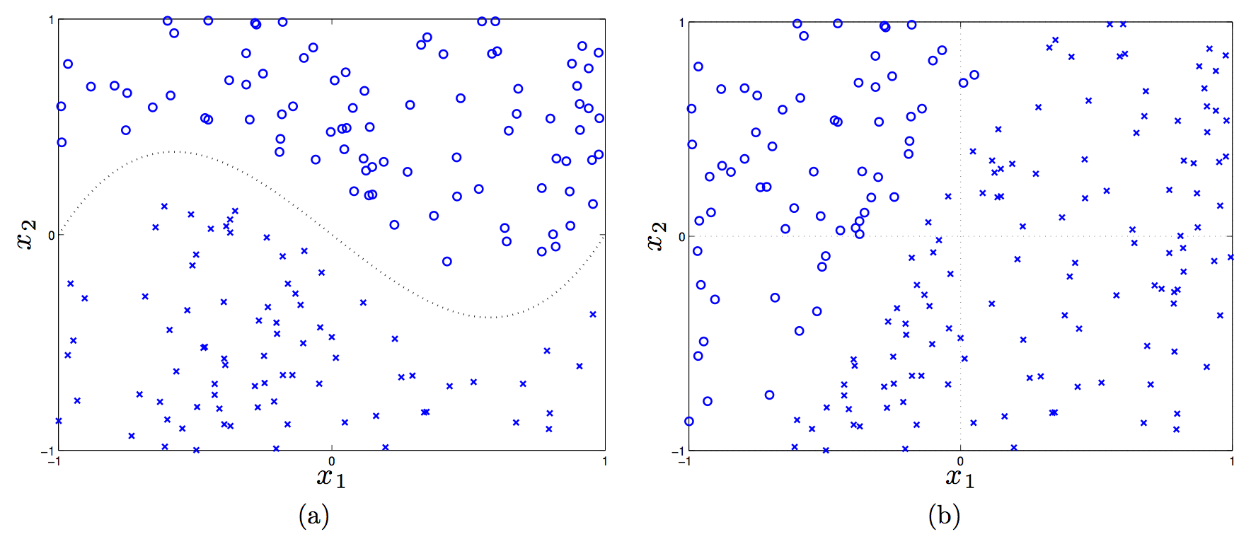
(In the first plot, the dotted line is \(f(x_1) = x_1^3 - x_1\).)

Let’s consider a linear, a shifted linear, a quadratic, and cubic kernels (see the handout for details on these), and see if any of them can linearly separate the data in the two plots.

Plot (a) requires a third-order polynomial to separate the data, so only the cubic kernel will work, because that will map feature vectors \(x \to \phi(x)\) to have \(x_1^3\) in it. Then we’d just adjust the weights to set that to have nonzero weight.

In plot (b), a linear kernel is enough, but there has to be a bias term in there! (That actually tricked me.) Without a bias, in the 2-D case here, the decision rule is \({\rm sign}(w^Tx)\), and a 2-D vector \(w\) must “emanate” out of the origin, which means the perpendicular line to it crosses the origin.

Kernels, Formalized

The preceding discussion motivates the following question: how do we know if a function \(K\) is a valid kernel? First, the official definition of a kernel is that it is a function \(K(x,y) = \phi(x)^T\phi(y)\) that performs an inner product in a Hilbert Space. Normally, I prefer thinking of the inner product \(\langle \phi(x),\phi(y) \rangle\) as the normal dot product (as I wrote earlier) but more generally, we should use the terminology of the inner product. Those satisfy properties of symmetry, bilinearity, and positive definiteness. A Hilbert Space is an inner product space that is complete and separable with respect to the norm defined by the inner product.

Since we are only dealing with real-valued vectors, our Hilbert Space will be \(\mathbb{R}^n\) and the inner product here is the normal vector dot product. To test whether a function is a kernel, we invoke a simplified form of Mercer’s Theorem: let function \(K : \mathbb{R}^n \times \mathbb{R}^n \to \mathbb{R}\) be given. Then for \(K\) to be a valid Mercer kernel, it is necessary and sufficient that for any set of points \(\{x^{(1)}, \ldots, x^{(m)}\}\) the corresponding kernel matrix is (symmetric) positive semi-definite. The element \(K_{ij}\) of the kernel matrix is the value \(K(x^{(i)},x^{(j)})\). (Sometimes the kernel matrix is called the Gram matrix.)

To prove one direction, that if \(K\) is a kernel matrix corresponding to a feature mapping \(\phi\), it must be symmetric positive semi-definite, we proceed as follows. First, it’s going to be symmetric due to the dot product (or more accurately, inner product) being commutative. Next, for any \(z \in \mathbb{R}^n\), we have

\[\begin{align} z^TKz &= \sum_{i=1}^n\sum_{j=1}^n K_{ij}z_iz_j \\ &= \sum_{i=1}^n\sum_{j=1}^n z_i \phi(x^{(i)})^T\phi(x^{j})z_j \\ &= \sum_{i=1}^n\sum_{j=1}^n z_i \sum_{k=1}^n \phi_k(x^{(i)})\phi_k(x^{j})z_j \\ &= \sum_{k=1}^n\sum_{i=1}^n\sum_{j=1}^n z_i \phi_k(x^{(i)}) \phi_k(x^{(j)}) z_j\\ &= \sum_{k=1}^n \left( \sum_{i=1}^n z_i\phi_k(x^{(i)})\right)^2 \ge 0 \end{align}\]

where we used the fact we indirectly showed earlier that \(\sum_i\sum_j x_iz_ix_jz_j = (x^Tz)^2 \ge 0\). It’s a little tricky because we are keeping \(k\), a component of \(\phi\), fixed, and ranging across different \(\phi\) vectors.

This fact about positive semi-definiteness makes it easy to see that the following are also valid kernels:

• Addition: \(K_1 + K_2\)
• Multiplication: \(K^T K\)
• Scalar: \(cK\) for a constant \(c \ge 0\)

We can use kernels for perceptrons (as previously discussed), support vector machines (as we will discuss), principal components analysis, and other classifiers such as linear regression.

Let’s discuss the linear regression case. In the general (regularized) case, the objective is:

\[\arg_w \min \|y - Xw\|_2^2 + \lambda \|w\|_2^2\]

where \(X\) is the \(n \times m\) matrix of training instances, where each training instance is a row (this is different from what I usually think of it, but it makes more sense in regression). The \(y \in \mathbb{R}^n\) vector has the true labels. By taking derivatives, we see that the optimal \(w\) is

\[w = (X^TX + \lambda I)^{-1}X^Ty = X^T(XX^T + \lambda I)^{-1}y\]

In the last step above, I used the clever trick I learned from CS 281A that for \(\lambda > 0\) and a matrix \(A\) that is \(d\times n\), we have \((AA^T + \lambda I)^{-1}A = A(A^TA + \lambda I)^{-1}\). But wait, what does this mean? We can express \(w\) as

\[w = X^T(XX^T+\lambda I)^{-1}y = \sum_{i=1}^n \alpha_i x_i\]

with an appropriately defined \(\alpha_i\) since the columns of \(X^T\) (not \(X\), be careful!) are the actual training elements, so \(w\) is in the space spanned by them and thus we can write it as a linear combination.

When we are faced with a new training instance to do regression, \(x_{\rm new}\), we will perform the following:

\[f(x_{\rm new}) = (x_{\rm new})^Tw = (x_{\rm new})^T \left(\sum_{i=1}^n \alpha_i x_i \right) = \sum_{i=1}^n \alpha_i \langle x_i, x_{\rm new}\rangle\]

We have kernels again! This is more accurately known as kernelized linear regression. In fact, we even use kernels before we test on new examples (i.e., we use it during training). Why? The matrix \(XX^T\) is itself a kernel matrix! It consists of dot products between the training instances, and since we optimize over that during training, we will use kernels during training.

I may end up reading more of Tom Mitchell’s slides on this, because this was quite illuminating to me.

Support Vector Machines

We now switch gears to Support Vector Machines (SVMs), which are possibly the best “off-the-shelf” classifier because they combine the kernel trick along with the concept of a maximum margin separator. Thus, we know immediately that – like in the perceptron – we must find some way to express the optimization problem in terms of dot products.

To begin the derivation, we define the functional margin of a weight vector \((w,b)\) (note: we keep the intercept term separate now) with respect to training instance \(x^{(i)}\) to be \(\gamma^{(i)} = y^{(i)}(w^Tx^{(i)}+b)\), where the class label \(y^{(i)} \in \{-1,1\}\), and across the entire dataset, \(\gamma\) is just the minimum of all the functional margins. Ideally, we would like the functional margin to be relatively large, as that would indicate a strong, “robust” boundary between the two classes.

We can formulate SVMs with the following “optimization” problem:

\[\max_{\gamma,w,b} \gamma\]

such that

\[y^{(i)}(w^Tx^{(i)}+b) \ge \gamma,\quad \forall i\]

along with the restriction that \(\|w\|_2 = 1\), which prevents the functional margin from changing due to invariance of the size of \(w\) (though \(b\) might vary, but I don’t think it’s a problem).

Unfortunately, this is not really possible with “optimization” easily, so we transform the problem into an equivalent one as follows:

\[\min_{w,b} \frac{1}{2}\|w\|_2^2\]

such that for all training instances \(i \in \{1,2,\ldots,m\}\), we have the constraint \(y^{(i)}(w^Tx^{(i)} + b) \ge 1\). This scales \(w,b\) so that the functional margin must be one.

We are done, but it is better to face the problem from the dual perspective so that we can take advantage of kernels. Since the dual solution \(d^*\) is less than or equal to the primal solution \(p^*\), it follows that we can equivalently solve the problem by maximizing the dual⁴. We re-write the constraints as \(g_i(w) = 1-y^{(i)}(w^Tx^{(i)}+b) \le 0\) and construct the Lagrangian as:

\[\mathcal{L}(w,b,\alpha) = \frac{1}{2}\|w\|_2^2 - \sum_{i=1}^{m} \alpha_i (y^{(i)}(w^Tx^{(i)}+b) - 1)\]

Setting the derivative of \(\mathcal{L}\) with respect to \(w\) and \(b\), then after some algebra (which took me a while due to lots of indices messing me up, but I eventually got it), and then knowing that we need to maximize this, we pose the dual optimization problem:

\[\max_\alpha \sum_{j} \alpha_j - \frac{1}{2}\sum_{j}\sum_{k} \alpha_j \alpha_k y^{(j)} y^{(k)}(x_j^T x_k)\]

such that \(\alpha_i \ge 0\) for all \(i\), and \(\sum_{i=1}^m \alpha_iy^{(i)} = 0\). Fortunately, this is convex, so there is a single global minimum.

Notice that we have \(\alpha\) variables again, though these have a different interpretation than the ones in the kernelized perceptron, though. Watch out! And yes, we do get kernels to appear once again. Nice!

Now let’s see what happens when we have trained and are going to assign a class to a new instance \(x_{\rm new}\). We perform the \({\rm sign}(w^Tx_{\rm new}+b)\) computation, which can equivalently be expressed as

\[w^Tx_{\rm new}+b = \left(\sum_{i=1}^m \alpha_i y^{(i)}x^{(i)}\right)^Tx_{\rm new} + b = \sum_{i=1}^m \alpha_i y^{(i)} \langle x^{(i)},x_{\rm new}\rangle + b\]

Once again, we have kernels! Incidentally, it looks like we might have to do a lot of computation for classifying a single point, but in fact, most of the \(\alpha_i\)s will be zero. The few that are nonzero correspond to the training instances called support vectors, and they are the ones closest to the margin. This is formally called the Karush-Kuhn-Tucker dual complementarity condition. The fact that we may not need to do much computation means SVMs gain some of the advantages of parametric models.

In the above problem, we – just like in the kernelized perceptron and kernelized regression – have formulated the problem so that, both during training and classification of new examples, the data enter via inner products, allowing us to use kernels.

What happens when we do not have linearly separable data? Rather than come up with a more complicated or longer feature vector (which might risk overfitting), we can reformulate the problem using slack variables (for \(\ell_1\)-regularization) and an additional, controllable parameter \(C\):

\[\min_{w,b} \frac{1}{2}\|w\|_2^2 + C \sum_{i=1}^m \xi_i\]

such that for all \(i \in \{1,2,\ldots,m\}\), we have \(y^{(i)}(w^Tx^{(i)}+b) \ge 1 - \xi_i\) and \(\xi_i \ge 0\). Thus, samples are permitted to have a (functional) margin less than one.

Rather surprisingly, the only change to the dual is that \(\alpha_i \ge 0\) constraints turns into \(C \ge \alpha_i \ge 0\) constraints, so we can apply the same principles (roughly speaking) as we did in the linearly separable case. In addition, the way we find \(b\) changes, but generally we don’t really worry about the intercept too much when going through the derivation. It’s really \(w\) that matters most to me.

---

In this post, we’ll review Markov Decision Processes and Reinforcement Learning. This material is from Chapters 17 and 21 in Russell and Norvig (2010).

Markov Decision Processes

The general idea with this situation is that we are an agent in some world, and we have a set of states, actions (for each state), a transition probability (which we may not actually know), and a reward function. The goal for a rational agent is to maximize the expected sum of (discounted) rewards for a state \(\mathbb{E}[\sum_t \gamma^t R(s_t)]\), where \(0 \le \gamma \le 1\) is our discount factor, which we usually assume is equal to one for toy cases only.

This is the setup of a Markov Decision Process (MDP), with the added constraint that the probability of going to another state only depends on the current state, which is why we call this a Markov Decision Process. Since the ultimate goal is to maximize the expected utility, we will need to learn a policy function \(\pi\) that maps states to actions. Finally, while not strictly necessary, it is common to “spice up” the MDP problem by assuming that actions are non-deterministic. In the canonical grid-world example described in the book (and in a lot of undergraduate AI classes, for that matter), we assume if we move North, then that has an 80 percent chance of succeeding. Hence, the transition probability \(P(s' \mid s, a) = P(s,a,s')\) is nontrivial, where \(s\) and \(s'\) are states, and \(a\) is the action we took at state \(s\).

In order to understand how to get an optimal policy, we first need to realize how exactly to define the value \(V^*(s)\) of a state, which in other words, is the expected utility we will get if we are at state \(s\) and play optimally. (The asterisk here is to indicate optimality.) There are, sadly, two common formulations for \(V^*(s)\). The first, from R & N, assumes that the reward aspect of the formula is defined in terms of a state only:

\[V^*(s) = R(s) + \gamma \max_a \sum_{s'} P(s,a,s') V^*(s')\]

The second formulation, which Berkeley’s CS 188 class uses¹, defines reward in terms of a state-action-successor triple:

\[V^*(s) = \max_a \sum_{s'} P(s,a,s') [R(s,a,s') + \gamma V^*(s')]\]

Both of these equation sets can be called the Bellman Equations, which characterize the optimal values (but we will generally need some other way of computing them, as we show shortly). In general, I will utilize the second formulation, but the formulations are not fundamentally different.

It is also common to define a new quantity called a Q-value with respect to state-action pairs:

\[Q^*(s,a) = \sum_{s'} P(s,a,s')[R(s,a,s') + \gamma V^*(s')]\]

In words, \(Q(s,a)\) is the expected utility starting at state \(s\), taking action \(a\), and hereafter, playing optimally. We can therefore relate the \(V\)s and \(Q\)s with the following equation:

\[V^*(s) = \max_a Q^*(s,a)\]

I find it easiest to think of these in terms of expectimax trees with chance nodes. The “normal” nodes correspond to \(V\)s, and the “chance” nodes correspond to \(Q\)s. Both nodes have multiple successors: the \(V\)s because we have choices of actions, and \(Q\)s because, even if we commit to an action, the actual outcome is generally non-deterministic, so we will not know what state we end up in. (I guess we can also view states as the “normal” nodes here.)

Given these definitions, how do we figure out the optimal policy? There are two common tactics:

• Value Iteration is an iterative algorithm that computes values of states indexed by a \(k\), as in \(V_k(s)\), which can also be thought of the best value of state \(s\) assuming the game ends in \(k\) time-steps. This is not the actual policy itself, but these values are used to determine the optimal policy².

  Starting with \(V_0(s) = 0\) for all \(s\), value iteration performs the following update:

  \[V_{k+1}(s) \leftarrow \max_a \sum_{s'} P(s,a,s') [R(s,a,s') + \gamma V_{k}(s')]\]

  and it repeats until we tell it to stop.

  To make this intuitive, during each step, we have a vector of \(V_k(s)\) values, and then we do a one-ply expectimax computation to get the next vector. Note that expectimax could compute all of the values we need, but it would take too long due to repeated and infinite depth state trees.

  To prove value iteration converges to \(V^*\) (and uniquely!), appeal to contraction and the fact that \(\gamma^k\), so long as \(\gamma \ne 1\), will go down to zero. Said another way, the “\(V_k\) tree” and the “\(V_{k+1}\) tree” are different only in their last layer, but that last layer’s contribution is reduced exponentially.

• Policy Iteration is generally an improvement over Value Iteration because policies often converge long before the values do, so we alternate between policy evaluation and policy improvement steps. In the first step, we assume we are given a policy \(\pi\) and have to figure out the expected utilities of each state when executing \(\pi\). These values are characterized by the following equations:

  \[V^\pi(s) = \sum_{s'} P(s,\pi(s),s') [R(s,\pi(s),s') + \gamma V^\pi(s')]\]

  Note that the MAX operator is gone because \(\pi(s)\) gives us our action. Thus, we can solve these equations in \(O(n^3)\) time with standard matrix multiplication methods³.

  It is actually rather easy to do policy improvement from Q-values:

  \[\pi^*(s) = \arg_a \max Q^*(s,a)\]

  Alternatively, we can use the more complicated expectimax form:

  \[\pi^*(s) = \arg_a \max \sum_{s'} P(s,a,s')[R(s,a,s') + \gamma V^*(s')]\]

  The two steps would iterate until convergence, and like value iteration, policy iteration is optimal. Also, these equations are really policy extraction, in the sense that given values, we know how to get a policy.

In general, policy iteration seems to be a slightly better bet than value iteration, though I guess the latter could be simpler to implement in some cases since it only involves the value updating part?

If we do not know exactly what state we are in, we do not have a notion of \(s\) here, so we need to change our representation of the problem. This is the Partially Observable Markov Decision Process (POMDP) case. We augment the MDP with a sensor model \(P(e \mid s)\) and treat states as belief states. In a discrete MDP with \(n\) states, the belief state vector \(b\) would be an \(n\)-dimensional vector with components representing the probabilities of being in a particular state. The belief state update for a particular component (state) \(s'\) looks a lot like an HMM update:

\[b(s') \propto P(e \mid s') \sum_{s'} P(s' \mid s, a) b(s)\]

The cycle is: we compute an action from \(b\), see evidence \(e\), compute a new belief state (using the above formula), then repeat. Fortunately, the optimal action for a POMDP only depends on the current belief state, allowing us to have our policy \(\pi\) be a mapping from a belief state to an action.

We can also map POMDPs to an observable MDP formula, by appropriately defining transition \(P(b' \mid b, a)\) and reward \(\rho(b)\) functions. For instance, \(\rho(b) = \sum_{s}b(s)R(s)\). The optimal policy for this new MDP over the belief states is the same optimal policy over the original POMDP. This is good, since we’ve reduced this problem to an MDP, but we have to modify our earlier algorithms to handle continuous-valued state spaces. A key observation that will help: the value function \(V(b)\) over belief states is piecewise linear and convex, because it is the maximum of a collection of hyperplanes. What a modified value iteration algorithm needs to do is to accumulate a set of possible plans, and for a given belief state, compute which of those has the optimal hyperplane. But this is too slow so in practice, people use online algorithms based on one-step lookahead, inspired by Dynamic Bayesian Networks.

To understand POMDPs well, consider simple MDPs with two states, so we can represent \(b\) as a scalar.

Reinforcement Learning

Now we switch to the reinforcement learning case. Before diving into the details, it is easiest to think of us in the same MDP framework, except that we have to learn our policy online, not offline. This is harder because we typically assume we do not know the transition probabilities ahead of time, or even the rewards. Unfortunately, this means we will try out different paths, and will sometimes fail (e.g., falling into the -1 pit in the gridworld example).

First, consider the passive reinforcement case, where we are given a fixed (possibly garbage) policy \(\pi\) and the only goal is to learn the values at each state, according to the Bellman equations.

Here’s one way to get the values: learn the transitions \(P\) and the rewards \(R\) through trials, then immediately apply the policy evaluation step in policy iteration. As a reminder, this computes values (as in value iteration) but since the policy is fixed, we can solve the set of equations quickly. This technique, which Russell and Norvig seem to call adaptive dynamic programming, is part of the class of model-based learning techniques, because that assumes we have to compute a model of the world (i.e., the transitions and rewards). Here, our agent could play a series of actions from a variety of states (“restarting” when necessary). At the end, it will have data about the rewards it’s gotten, along with the number of times it transitioned from state \(i\) to state \(j\). To compute the transition function, we would convert the counts to the averages in a “Maximum Likelihood Estimate”-manner. The rewards are easier because we can see \(R(s,a,s')\) immediately when we transition from \(s\) to \(s'\).

In model-free learning, we do not bother to compute the transition model, but instead only compute the actual values of each state. There is a basic technique called direct utility estimation that falls in this category of methods. The idea here is that for each trial, we need to record the sum of discounted rewards for each state visited. After a series of trials, these values will average out and converge, albeit slowly since direct utility estimation does not take into account the Bellman Equations.

We need a better solution. Since we already have a policy, we would like to do some form of policy evaluation (explained earlier), but we do not have the transitions and rewards. We can approximate those with our samples instead, which leads to Temporal Difference learning. This is a model-free tactic where, after each transition \((s,a,s',r)\), we update the values:

\[V^\pi(s) \leftarrow (1-\alpha)V^\pi(s) + \alpha\underbrace{[R(s,\pi(s),s') + \gamma V^\pi(s)]}_{\rm sample}\]

In short, TD learning works by adjusting the utility estimates towards the ideal equilibrium as stated by the Bellman equations. But what if we want to get a new policy? TD learning does not learn the transition probabilities, so we switch to learning Q-values, since it is easier to extract actions from Q-values.

This now brings us to active reinforcement learning, where we have to learn an optimal policy by choosing actions. Clearly, there will be some tradeoffs between exploration and exploitation.

The solution here is an algorithm called Q-Learning, which iteratively computes Q-values:

\[Q(s,a) \leftarrow (1-\alpha) Q(s,a) + \alpha \underbrace{[R(s,a,s') + \gamma \max_{a'}Q(s',a')]}_{\rm sample}\]

Notice how the sample here is slightly different than in TD learning. Each sample is computed from a \((s,a,s',r)\) tuple.

The amazing thing is, so long as certain obvious assumptions hold, such as that we visit states sufficiently often, Q-Learning will converge to an optimal solution even if the actions we take are repeatedly suboptimal⁴! In the fire pit example in the CS 188 class, we could keep jumping in the pit, but so long as our actions are somewhat stochastic, we will eventually have some paths that end up in the lone beneficial spot, which will result in higher Q-values for those states and actions that lead towards that spot. (Think of each grid as having four Q-values.)

Even so, it would probably be wise to have good heuristics for deciding on what actions to take, which might make Q-Learning converge faster. The simplest (and worst) strategy: act according to a current policy, but with some small probability, we choose a random action. To improve this, use exploration functions that weigh the importance of actions and states based on whether their values are “established” or not. This information propagates back so that we end up favoring actions that lead to unexplored areas. This means for some exploration function \(f\), the action we pick at a step will be \(\arg_{a'} \max f(Q(s',a'), N(s',a'))\) where \(N\) represents counts, and the new Q-Learning update is:

\[Q(s,a) \leftarrow (1-\alpha) Q(s,a) + \alpha \underbrace{[R(s,a,s') + \gamma \max_{a'} f(Q(s',a'), N(s',a')]}_{\rm sample}\]

There is a close relative to Q-Learning called SARSA, State-Action-Reward-State-Action. The update is, following Russell and Norvig’s notation to have rewards be fixed to a state:

\[Q(s,a) \leftarrow (1-\alpha)Q(s,a) + \alpha(R(s) + \gamma Q(s',a'))\]

What this means is that we already have an action \(a'\) chosen for the successor state \(s'\). Q-Learning will choose the best action \(a'\), but in SARSA, it is fixed, and then we can update \(Q(s,a)\). SARSA and Q-Learning (the first version here, not the second version with \(f\)) are the same for a greedy agent always picking the best action. When exploration happens, Q-Learning will attempt to pick the best action, but SARSA picks whatever is actually going to happen. This means Q-Learning does not pay attention to the policy, i.e., it is off-policy, but SARSA does, so it is on-policy. Here’s an example I thought of to clarify: the fire pit in CS 188 means that a policy that tells us to go in the pit will be bad, but if transitions are stochastic, then at some point, we will get to the good exit, hence Q-Learning will eventually learn that best value. But with SARSA, we do not get that opportunity because we will always have the next action fixed, so it is “more realistic” in some sense.

It is worth pointing out that all this previous discussion about learning all the \(Q(s,a)\) values is really applicable only for the smallest of problems, because we cannot tabulate all those in real-life situations. Thus, we resort to Approximate Q-Learning. Here, we use feature-based representations by representing a state as a vector of features:

\[V(s) = w_1f_1(s) + \cdots + w_nf_n(s)\]

And the same for the Q-values:

\[Q(s,a) = w_1f_1(s,a) + \cdots + w_nf_n(s,a)\]

We usually make things linear in terms of the features for simplicity. This has the additional benefit in that we can generalize to states we have not visited yet (in addition to the obvious compression benefits). Note that when we do the Q-Learning update here, we change the weights. Each weight update looks like the same kind of update we see in stochastic gradient descent.

Finally, the last major reinforcement learning topic is policy search. It actually seems like the policy iteration analogue: we only care about the policy, not the actual values themselves. Starting with an initial feature-based representation of the Q-states, we might consider tweaking the individual weights up and down and then evaluating the result of that representation to see if our rewards are higher. This may involve computing an expression for the expected reward, or running an agent in the world multiple times.

Old CS 188 Exam Questions

I found four interesting questions related to MDPs and reinforcement learning.

• Spring 2011, Question 4 (“Worst-Case Markov Decision Processes”). Now we measure the quality of a policy by its worst-case utility, or in other words, what we are guaranteed to achieve. This question is really intellectually simulating, as we have to consider the algorithm from a minimax perspective, rather than an expectimax perspective.

  For a state, we have:

  \[L^*(s) = \max_a \min_{s' \in C(s,a)} [R(s,a,s') + \gamma L^*(s')]\]

  So we pick the action that maximizes the following quantity: it is the discounted reward based on the worst possible state \(s'\) to which we could transition.

  There is a corresponding Q-value version:

  \[M^*(s,a) = R(s) + \gamma \min_{s' \in C(s,a)} \max_{a'} M^*(s',a')\]

  We are guaranteed \(R(s)\), but have already committed to action \(a\), so the adversary is free to send us to the worst possible subsequent state for us (as long as that transition has non-zero probability, of course), but then we are free to maximize over the next action.

  If we want to do \(M\)-Learning, then it is actually easier than standard \(Q\)-Learning because the environment has deterministic rewards and we only care about the minimax one, so if we ever observe a reward, we know that it’s the correct one.

• Fall 2011, Question 4 (An un-named question). This one required us to actually perform some computations of value iteration and Q-learning. The only non-trivial thing about this was the jump from C, which could land in either D or E. I personally found it easiest to just run Value Iteration and try to reason about the Q-values later. The Q-learning iterative update is:

  \[Q_{k+1}(s,a) \leftarrow \sum_{s'} P(s,a,s') [R(s,a,s') + \gamma \max_{a'}Q_k(s',a')]\]

  For the third part, the tricky thing was to remember that the Q-learning update will involve MAX-ing over previously computed Q-values.

• Fall 2012, Question 6 (“Reinforcement Learning”). This question makes clear the distinction between Q-Learning and SARSA. For part (a), they give us the formula for the Q-Learning agent, and ask if this will converge to the optimal set of Q-values even if the policy we’re following is suboptimal. The answer is yes, since they also mention in the question several necessary requirements (e.g., that we visit all state-action pairs infinitely often). For part (b), the SARSA update, answer is no, we do not converge to the optimal Q-values, because SARSA will have Q-values for whatever policy is actually being executed. This policy that we converge to is the policy that follows \(\pi\) with probability 0.5, and uniformly random otherwise.

• Fall 2012, Question 7 (“Bandits”). This is a rather long question. Part (a) gives a nice review of MEU and VPI, and the remaining parts now deal with POMDPs over the two states of having bandits versus not having bandits. Hence, we represent the belief state as a single scalar \(b\) representing the probability we believe there are bandits. When we have to compute \(b_{t+1} = P(s_{t+1} = +b)\) in the tree, we use the following formula:

  \[P(s_{t+1} = +b) = \frac{P(e = +safe \mid s_{t+1} = +b)b_t}{P(e = +safe \mid s_{t+1} = +b)b_t + P(e = +safe \mid s_{t+1} = -b)(1-b_t)}\]

  Notice that this is precisely the formula for updating the belief state that we discussed earlier in the notes, except that we have the transition function as the identity. By the way, it took me a while to figure this out, but the normalizing constant here needs to iterate through the set of belief states. We have a scalar \(b_t\), but we really have to consider the case of there possibly being no bandits at all. A bit tricky here. The transition probability is also tricky, so it’s easiest to think of it in terms of the problem: what is the probability of even reaching this node?

  Finally, they discuss some utility diagrams. As we discussed earlier, to find the overall value function, we take the maximum over all the possible lines. For the discounting questions, part (i) the point was that agents with larger \(\gamma\) values should be more concerned about the future, so they are more willing to try out short-term suboptimal paths. Thus, Agent A has a higher discount factor because it played the sub-optimal Land action one more time. In part (ii), there are three plots you can easily remove. Then it’s just assigning three plots to three discount factors. A higher discount factor means we need to be more certain that we have bandits before we commit to making air shipments.

---

After reviewing some linear algebra, the Least Mean Squares (LMS) algorithm is a logical choice of subject to examine, because it combines the topics of linear algebra (obviously) and graphical models, the latter case because we can view it as the case of a single, continuous-valued node whose mean is a linear function of the value of its parents. (Admittedly, I do not find this intuitively helpful.)

The High-Level Problem

We are going to be analyzing LMS in the context of linear regression, i.e., we will have some input features \(x_n = (x_1, x_2, \ldots, x_k)^{(n)}\) along with their (scalar-valued) output \(y_n\) as our data, and the goal is to estimate a parameter vector \(\theta\) such that \(y_n = \theta^T x_n + \epsilon_n\), where the \(\epsilon_n\) is admitting that we do not expect to exactly match \(y_n\).

When we have ordinary linear regression, we often express the data all together in terms of matrices. Thus, we could have \(X\) be our \(m \times n\) matrix of features, where there are \(m\) samples and \(n\) variables per sample, \(\theta\) be the \(n\times 1\) column vector of parameters, and the goal would be to find a solution \(\theta\) to the problem \(X\theta = Y\), where \(Y\) is the column vector of actual outputs. The problem is linear because the equations are linear in \(\theta\) (\(X\) itself can actually be input to a more complicated function). In the rare case that \(X\) is square and that all columns are linearly independent, this immediately reduces to \(\theta = X^{-1}Y\). Most of the time, though, \(X\) is a “tall” matrix and the data vector \(Y\) lies outside the column space of \(X\).

The most natural solution, it seems, is to find the projection of \(Y\) onto the subspace of \(Col(X)\), as that intuitively should minimize all our \(\epsilon_n\) terms. Thus, we have the normal equations, the most important one in statistics: \((X^TX)\theta = X^TY\). In most cases¹, we can invert \((X^TX)\). If not, we can use the pseudo-inverse².

There are several ways of getting to the normal equations. One can appeal geometrically, by using geometry and linear algebra. Alternatively, we can derive it based on the following cost function:

\[\begin{align} J(\theta) &= \frac{1}{2}\sum_{n=1}^N \epsilon_n^2\\ &= \frac{1}{2} \sum_{n=1}^N (y_n - \theta^Tx_n)^2 \\ &= \frac{1}{2} (y - X\theta)^T(y - X\theta)\\ &= \frac{1}{2} \|y - X\theta\|_2^2 \end{align}\]

If someone asks you about what LMS (which we will discuss shortly) is supposed to optimize, it is this cost function. We want to minimize the sum of squared errors.

So, under the assumption that we can get \(\theta\) by inverting \(X^TX\), we can solve this via direct methods (e.g., Gaussian elimination) or iterative methods. The latter is our focus, as the LMS algorithm is an example of an iterative method. Put another way, it is a steepest descent algorithm for solving the normal equations.

The LMS Algorithm

The gradient of the cost function³ over all the data (i.e., the “batch” case, not the “online” case) leads to the update rule:

\[\theta^{(t+1)} = \theta^{(t)} + \rho \underbrace{\sum_{n=1}^N(y_n - (\theta^{(t)})^T x_n)x_n}_{\nabla J(\theta)}\]

We just initialize some \(\theta^{(0)}\) and run this until convergence. But this is bad because we are summing up over the entire set of samples. Thus, we use the following single-case update, which is indeed what we mean by the LMS algorithm:

\[\theta^{(t+1)} = \theta^{(t)} + \rho \underbrace{(y_n - (\theta^{(t)})^T x_n) x_n}_{\nabla_{x_n} J(\theta)}\]

In other words, the idea is that we take each data point stochastically⁴, which provides an approximation of the gradient, in the hopes that \(\theta\) will converge to whatever is implied by the normal equations. The above equation is the LMS update. While LMS is technically an approximation, it is in fact often superior to the batch version equation update written earlier.

This update rule has the following neat, intuitive interpretation courtesy of Michael I. Jordan. Suppose we are given \((x_n,y_n)\); what update should we perform on \(\theta\)? If this is our only data, then we have vectors \(x_n\) and \(\theta\) in some space. To map \(\theta^Tx_n\) perfectly onto \(y_n\), we must figure out a way to project⁵ \(\theta\) onto \(x_n\). In general, there will be a line of possible solutions for \(\theta\), but the two “natural” ways to update \(\theta\) are by extending \(\theta\) in either (1) the “\(\theta\) direction” or (2) the “\(x_n\) direction.” The second case is easiest to do because the error associated with the projection of \(\theta\) is precisely \(x_n - y_n\), and by projecting \(\theta\) by this amount in the direction of \(x_n\), we will get \(y_n = \theta^Tx_n\) with no error term. In general, the rule will be:

\[\theta^{(t+1)} = \theta^{(t)} + \frac{1}{\|x_n\|_2^2}(y_n - (\theta^{(t)})^Tx_n)x_n\]

and this nicely maps to the LMS algorithm (in fact, it is the LMS algorithm update!) as we can turn the reciprocal of the norm term into \(\rho\). If we have multiple data points, we should expect the “jumping \(\theta\)” to eventually land at the solution, if there is one, or converge under certain conditions. The above equation means that we update \(\theta\) by moving it some distance in “the \(x_n\) direction.”

What I found especially interesting is that we can literally treat the parameter estimation \(\theta\) problem as a geometric problem, where each data point \((x_n,y_n)\) presents a constraint, and the overall goal is to solve a constraint satisfaction problem, a popular subfield in classic Artificial Intelligence.

It is possible to prove that LMS converges to a vector that satisfies the normal equations. I will not put the proofs here⁶, but it is important to understand these to see how much flexibility we have with the step size \(\rho\).

Side Notes

If we want to do weighted least squares, where each point is assigned a weight \(w_n\) that indicates its importance, then the cost function is \(J(\theta) = (1/2)(y-X\theta)^TW(y-X\theta)\), meaning that the normal equations turn into \(X^TWX\theta = X^TWy\). Our new matrix \(W\) is a diagonal matrix of weights.

We can connect our geometric treatment of LMS with probability. Suppose we endow the errors \(\epsilon_n\) as IID zero-mean Gaussians with variance \(\sigma^2\). Then, if we try to compute \(p(Y\mid X,\theta)\) for the entire data, what happens is that the log likelihood of this expression is equivalent to the least squares cost function \(J(\theta)\)! Said another way, maximizing the log likelihood with \(\theta\) is the same as minimizing the least-squares cost function, and all we assumed are IID sampling and Gaussian errors. Thus, we can avoid most of our geometric, constraint satisfaction approaches in favor of just computing the data log likelihood, since they evidently get the same results. This is assuming we stay in the maximum likelihood framework, by the way; the least-squares cost function can lead to a frequentist “estimator”, regardless of whether or not the data errors are Gaussian, and then that estimator and the MLE would not coincide. But here, they do.

It’s interesting to consider the question as to whether we can use LMS as discussed here for classification. As it is, it’s not a good fit for the classification case, but if we wanted to, we could adapt it into logistic regression. Then what this means is our hypothesis will still involve some form of \(\theta^Tx_n\), but we will instead use the logistic function:

\[h_\theta(x) = \frac{1}{1 + e^{-\theta^Tx_n}}\]

And the LMS would look like:

\[\theta \leftarrow \theta + \rho \left( y_i - \frac{1}{1+e^{-\theta^Tx_i}} \right) x_i\]

How do we derive this? Take the gradient of the log likelihood of the data under our logistic regression assumption, and pick the \(i\)th element.

It’s important to realize what we’ve done here. We have a similar algorithm as before, except here the conditional expectation of \(y_i\) given \(x_i\) is not measured by \(\theta^Tx_i\) but rather by the logistic regression. Also, we’ve assumed a logistic function from the outset, and are trying to fit this to data. This is known as the discriminative form of learning. Alternatively, we could have a generative classifier, which would involve computing class conditionals \(P(x\mid y)\) and categorical \(P(y)\). But in those cases, we don’t need iterative algorithms because we can get maximum likelihood estimates easily.

For the multi-class case, use the softmax function. Also, this still converges to something “linear” in the sense that this kind of classifier partitions the space into pieces, and this “partitioning” process is done with hyperplane surfaces, which are linear.

I hope to discuss logistic regression in more detail in a future blog post. While I (and you?) wait, here is another source about the LMS algorithm, courtesy of Andrew Ng. A lot of his notes really make things clear!

---

I’ll take a break from the recent discussion on graphical models to go over some old linear algebra concepts. While there are many references on linear algebra designed to help a student re-learn what he or she may have forgotten, I found the handout from Stanford’s CS 229 (Machine Learning) class to be one of the best when considering the content, size, and clarity together. And despite being advertised as a review, it actually did teach me a lot. In college, I only took one linear algebra class, a basic introductory and proofs-based course¹. While I found it difficult when I was taking it, in retrospect, we did not go over that much material. Two things that really tricked me up when I first arrived in Berkeley were

• Positive Definite Matrices (and related to that, Singular Value Decomposition)
• Matrix Calculus (with gradients, Hessians, etc.)

These two concepts are used all the time in AI, and I really wish I could know them better. Thus, in this post, I’ll quickly go over some of the basic review concepts of linear algebra as presented in the Stanford handout, and then spend a little more time on those previously mentioned topics.

Basic Concepts and Matrix Multiplication

A few years ago, I kept getting confused between column and row vectors when I was reading machine learning literature, but now I know that all vectors are assumed to be columns by default. Also, when denoting row vectors, be careful that the transpose sign does not necessarily mean we are taking the corresponding column and then transposing it (as the notes say, the definitions of \(a_1\) and \(a_1^T\) are ambiguous).

Matrix multiplication is at the heart of linear algebra and what we do in AI. I find it easiest to reason about matrix multiplication by always checking the number of rows and columns of the matrices involved, and making sure they align correctly. But this handout made it easier for me to think of other ways to view how multiplication works. They describe four interesting ways of looking at matrix multiplication, of which the most interesting to me is when the product \(AB\) is expressed as the sum of outer products (between vectors).

Operations and Properties

Some interesting operations and properties of matrices:

• Any square matrix \(A \in \mathbb{R}^{n\times n}\) can be represented as a sum of a symmetric matrix and an anti-symmetric matrix, since \(A = .5 (A + A^T) + .5 (A - A^T)\).

• The trace is the sum of the diagonal elements of a matrix. Despite its seeming simplicity, the trace operator will actually be very useful in matrix calculus (the “trace trick”) and in the study of eigenvalues and eigenvectors, since the sum of the eigenvalues of a matrix equals the trace, even though the individual components being summed up generally have no relation.

• The norm of a vector \(\|x\|\) is like an informal measure of the distance. For some reason, these kept confusing me when I was trying to work on my undergraduate thesis, so it’s nice to see it formally treated here. There are several properties of norms, but in general, I tend to view norms of vectors as just the \(\ell_p\) norm. Also, when working with norms, make sure I know the Cauchy-Schwarz inequality: \(|x \cdot y | \le \|x\| \|y\|\).

• The rank of a matrix is equal to the number of its linearly independent columns (or rows). There are many implications of the rank; for me, the one I remember the best is that in order for an inverse to exist, a (square) matrix has to be full rank. If we generated a square matrix by filling in its values from a random number generator, then it will almost always have full rank.

• A square matrix \(U\) is orthogonal if \(U^TU = I\). This requires the columns of \(U\) to be orthonormal². A nice property: \(\|Ux\|_2 = \|x\|_2\), which we can prove by squaring them, thus considering \((Ux)^T(Ux)\) and \(x^Tx\).

• The range, i.e., column space, of a matrix \(A \in \mathbb{R}^{m \times n}\) is \(\mathcal{R}(A) = \{v \in \mathbb{R}^m \: : \: v = Ax, x \in \mathbb{R}^n \}\). The null space is \(\mathcal{N}(A) = \{x \in \mathbb{R}^n \: : \: Ax = 0\}\)³. Vectors in the former set have length \(m\), those in the latter have length \(n\), and we can get the complement of each of those sets by considering \(\mathcal{R}(A^T)\) and \(\mathcal{N}(A^T)\). For instance, considering the sets \(\mathcal{R}(A^T)\) and \(\mathcal{N}(A)\), it turns out that the intersection of those two sets is empty, and that every vector in \(\mathbb{R}^n\) can be expressed as the sum of two vectors, one in each of those two sets. Thus, they are orthogonal complements. The two column spaces, combined with the two column spaces (using \(A\) and \(A^T\)) form the four fundamental subspaces, a term popularized by Gilbert Strang. I’m not sure I really get it, though.

• The determinant of a square matrix \(A\), denoted as \(det A\) or \(|A|\), is a mysterious function that maps \(A\) to the real numbers. The three main properties it satisfies are:

  • that the identity has determinant one
  • that if we multiply a single row in \(A\) by a scalar \(t\), the determinant of the new matrix is \(t|A|\)
  • that if we exchange any two (different) rows, then the determinant of the new matrix is \(-|A|\)

  All the other properties of determinants follow from this, including the cofactor expansion, which I will not list here. Determinants have an intuitive interpretation in terms of volume: if we take the span of the rows of \(A\), and restrict all the coefficients to be in \([0,1]\), then the determinant is the volume of this set. Also, determinants are useful for checking if \(A^{-1}\) exists. Finally, the adjoint of a matrix, \({\rm adj}(A)\), is \(A^{-1} = {\rm adj}(A) / |A|\).

• Given a square, symmetric matrix \(A\), a quadratic form is a function \(f(x) = x^TAx = \sum_{i=1}^n \sum_{j=1}^n A_{ij}x_ix_j\) mapping \(A\) and \(x\) to the reals. Our variables are \(x\), so even if the dimensions of \(A\) are large, the highest power of any \(x_i\) (i.e., a component of \(x\)) that can exist in \(f(x)\) is two, hence the intuitive name.

  Something that is related is the concept of a positive semidefinite matrix, which is a symmetric matrix such that \(x^TAx \ge 0\) for all \(x\). We can also define the obvious analogues for definite, negative definite, etc., matrices. Given any, not necessarily square matrix \(A\), the matrix \(A^TA\) is always positive semidefinite; prove this by using \(\|Ax\|_2^2\).

  Note: quadratic forms like these are the start of an introduction to what really happens in machine learning and AI, where we have to understand matrix representations.

• For determining eigenvalues and their corresponding eigenvectors (note: eigenvectors are not unique), refer to \({\rm det}(A - \lambda I) = 0\) if we are going to be solving them by hand.

  We tend to use \(\Lambda\) (capital lambda) to represent the matrix of eigenvalues, so the matrix equation will result in \(AS = S\Lambda\), implying that \(A = S\Lambda S^{-1}\), hence \(A\) is diagonalizable.

  Some interesting properties: the trace and determinant are the sum and product, respectively, of the eigenvalues. The eigenvalues of a triangular matrix are just the elements on the diagonal. If \(A\) is nonsingular, then \(1/\lambda_i\) is an eigenvalue of \(A^{-1}\) with eigenvector \(x_i\).

  If we have a symmetric matrix \(A\), then (1) all eigenvalues are real, and (2) its eigenvectors can be scaled to be orthogonal to each other, so that \(S\) above can turn orthogonal, and hence we have \(S^{-1} = S^T\), a good thing because transposes are easier computationally than inverses. Unfortunately, I don’t currently know how to prove these off the top of my head.

Singular Value Decomposition

With a symmetric matrix \(A\), we can set \(A = U\Lambda U^T\) instead of using \(U^{-1}\). It turns out we can generalize this to arbitrary (not even square!) matrices \(A\) by expressing them in singular value decomposition form, \(A = U\Sigma V^T\). The \(U\) and \(V\) matrices are square and orthogonal, and represent eigenvectors of \(AA^T\) and \(A^TA\), respectively.

The \(\Sigma\) matrix is diagonal, possibly non-square, and contains something called the singular values (not the eigenvalues!) of matrix \(A\). They fill the first \(r\) diagonal elements for a rank \(r\) matrix \(A\), and the rest of the elements are zero. The singular values are the square roots of the nonzero eigenvalues of both \(AA^T\) and \(A^TA\) (which are symmetric, so they have real eigenvalues).

For a positive definite matrix, \(U = V\).

There are many applications of SVD, and the ones I’m familiar with happen to be in computer vision. Some of these applications have to do with the fact that \(U\) and \(V\) give orthonormal bases for all four fundamental subspaces. For instance, to use SVD to compute the null space of \(A\), then look at the last \(n-r\) columns of \(V\).

Matrix Calculus

I really wish I had completely digested this section before taking CS 281A here because I had no idea how matrix calculus worked until I reviewed this document. Given a function \(f : \mathbb{R}^{m \times n} \to \mathbb{R}\), the gradient of \(f\) with respect to \(A\) is a matrix (i.e., it’s the same size as the original matrix input to \(f\)) of partial derivatives of \(f(A)\).

The Hessian is the second derivative analogue to the gradient (well, almost). Here, we assume we are taking the Hessian with respect to a function \(f : \mathbb{R}^n \to \mathbb{R}\), where we take a vector as input (not a general matrix, even though that’s possible).

The Trace Trick

Here’s a neat trick I learned from reading Mike Jordan’s notes. Since the trace is such that \(tr[ABC]\) is the same no matter what the ordering of the three matrices, and since \(\frac{\partial}{ \partial A} tr[AB] = B^T\) (verify this by explicit computation) then we can claim:

\[\begin{align} \frac{\partial}{\partial A} x^TAx &= \frac{\partial}{\partial A} tr[x^TAx] \\ &= \frac{\partial}{\partial A} tr[xx^TA] \\ &= \frac{\partial}{\partial A} [xx^T]^T = xx^T \end{align}\]

Intuitively, this makes sense since we just eliminated \(A\). In the past, when I tried computing derivatives like these, I would convert the entire expression to an enormous set of summations, and try to reason element by element. That is way too much work.

There is a related trick involving determinants: the derivative of \(\log |A|\) with respect to \(A\) is \(A^{-T}\).

One can use these tactics to take the MLE of the covariance matrix \(\Sigma\) of a multivariate Gaussian distribution, since the log likelihood of that term has \(\log |\Sigma|\) and \((x_n-\mu)^T\Sigma^{-1}(x_n-\mu)\) in it.

---

In this post, we will continue our discussion of graphical models by going over a special kind known as a Hidden Markov Model (HMM). These are appropriate for modeling forms of sequential data, implying that we finally relax various forms of “independent identically distributed” data or variables. They are a piece of the broader class of models known as Dynamic Bayesian Networks, of which Kalman Filters – which we will discuss in a future blog post here – are their continuous analogue.

Hidden Markov Models

HMMs are one of the most popular graphical models in real use (indeed, probably the most popular). They are characterized by variables \(X_1,X_2,\ldots,X_n\) representing hidden states and variables \(E_1,E_2,\ldots,E_n\) representing observations (i.e., evidence). The subscript \(i\) in \(X_i\) and \(E_i\) represents a discrete slice of time. There are three probability distributions in HMMs: a prior probability \(P(X_0)\), a transition probability \(P(X_t\mid X_{t-1})\) and an emission (sometimes called observation) probability \(P(E_t \mid X_t)\). That the transition probability only depends on the previous state means we are effectively invoking the Markov assumption. Whatever information about the state in the last time slice is all we need to know to determine the likelihood of the current state. Our distribution is stationary, which means that we only need to specify those three probabilities and we are set, because the CPTs are “carried over” to all the time slices. This is an instance of parameter tying.

There are several well-defined inference tasks and algorithms that we can conduct on HMMs, to which we now turn. True, we could simply take an HMM and run variable elimination on it, but the structure of HMMs provides us with some recursion we can exploit.

Filtering, Smoothing, and Predicting

These three are all similar. Given a series of observations, we want to determine the distribution over states at some time stamp. Concretely, we want to determine \(P(X_t\mid E_1,E_2,\ldots,E_n)\). The task is called filtering if \(t=n\), smoothing if \(t<n\), and predicting if \(t>n\). Clearly, smoothing will give better estimates, and prediction the weakest (or most uncertain) estimates.

To compute filtering estimates, we require a recursive computation. The actual algorithm we use is the forward algorithm. We will talk more about it later; here is the update equation for the forward algorithm:

\[P(X_{t+1} \mid e_{1:t+1}) \propto P(e_{t+1} \mid X_{t+1}) \sum_{x_t} P(X_{t+1} \mid x_t)P(x_t \mid e_{1:t})\]

where capital variables denote unknown variables, and the lowercase ones denote known variables. One can see that this equation makes intuitive sense. We sum up over all possible state realizations in the previous time step by their transition probability to the current state, and for each of those, we weigh the probability by the likelihood of emission from the state (which doesn’t depend on \(x_t\) so we can move it out of the sum). Furthermore, note that this is a recursive computation, a theme that will be common when we talk about inference in HMMs. Finally, the normalizing constant here is computed by summing up \(P(X_{t+1} \mid e_{1:t+1})\) for all possible realizations of \(X_{t+1}\). The normalizing is needed only because of the addition of the emission model probability downscaling our values.

Given that we know filtering, prediction is not that much more work, because we have the value up to the latest evidence variable, then it’s like we are ignoring the evidence variable and only using the transition probability:

\[P(X_{t+k+1} \mid e_{1:t}) = \sum_{x_{t+k}} P(X_{t+k+1} \mid x_{t+k}) P(x_{t+k} \mid e_{1:t})\]

(Here, we have no proportion sign.)

As we predict further into the distribution, we will eventually end up at the stationary distribution of the underlying Markov chain governing the sequence of state realizations. We can compute this as \(P\pi = \pi\), where \(P\) is the matrix of transitions, and \(\pi\) is the column vector of priors.

For smoothing, we actually need to compute something called a backward probability:

\[P(X_k \mid e_{1:t}) \propto \underbrace{P(X_k \mid e_{1:k})}_{f_{1:k}} \underbrace{P(e_{k+1:t}\mid X_k)}_{b_{k+1:t}}\]

The first component is what we were able to compute earlier, and we can do this recursively from the starting state. The second component is new, but in fact, it is not too hard to compute recursively – we just have to start backwards from \(t\). Here is the update:

\[P(e_{k+1:t}\mid X_k) = \sum_{x_{k+1}} P(e_{k+1}\mid x_{k+1}) P(e_{k+2:t}\mid x_{k+1}) P(x_{k+1}\mid X_k)\]

Notice now that we cannot move anything out of the summation, like we did with the forward update.

We can run something called the forward-backward algorithm, which will compute the forward probabilities, then the backward probabilities. We will return to these “forward” and “backward” subroutines in the following sub-sections, with two helpful figures representing these two algorithms.

The Likelihood of Observations

In this section, we’ll talk about two other common tasks in HMMs. The first is computing the likelihood of an observation sequence, \(P(e_{1:t})\). At first, it might not seem obvious how to do this, because we don’t even know the state sequence that caused the observations! Following the laws of probability, we have to include the states in our joint sequence, and then sum up over them. To do this efficiently, we use a dynamic programming algorithm called the forward algorithm, which folds together the paths that could have generated the observations.

I find it easiest to think of this computation just by looking at a trellis, like the one in the following image from Jurafsky’s book¹:

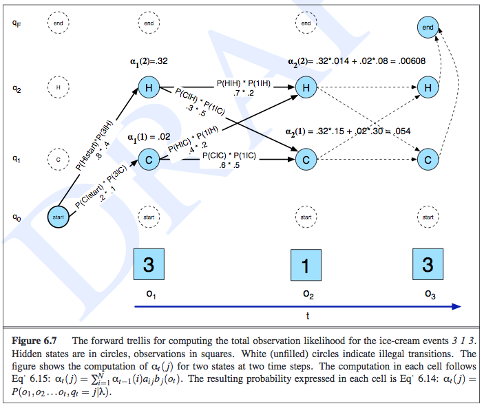
This example was about determining the observation likelihood of seeing three, one, and then three ice creams eaten in a day, and the state variables represented the temperature of the day. In the trellis, the rows correspond to the possible realizations of each state, along with one other row to symbolically represent the emission/observation/evidence. The notation of \(\alpha_t(j)\) represents the probability of the observation sequence and being at a particular state at time \(t\), so \(\alpha_t(j) = P(e_{1:t},x_t = j)\). The computation of \(\alpha\) is done recursively in an intuitive manner, as shown in the image:

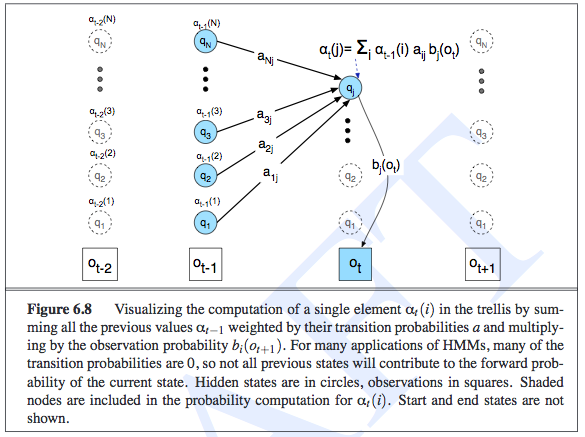
Intuitively, the likelihood of an observation sequence should be the sum of all the possible state sequences that could have led to that observation. The fact that we are summing up and storing probabilities in the previous \(\alpha_{t-1}\) terms is an indication of the HMM’s independence assumptions, and is what lets us do inference efficiently. Oh, and to actually compute the observations, we do need to sum out \(x_t\) from \(\alpha_t(j)\).

By the way, did you notice that these “updates” that we are doing are exactly what we did for the filtering step earlier? It’s just taking an earlier factor (representing whatever probability we want) and multiplying it by the transition and then the emission probability! In Russell and Norvig, the update equation is called \(z_{1:t+1} = {\rm FORWARD}(z_{1:t}, e_{t+1})\), and \(z_{1:t}\) can represent \(f_{1:t} = P(X_t \mid e_{1:t})\) or \(\ell_{1+t} = P(e_{1:t}, X_t)\). While \(f\) and \(\ell\) are clearly different, their updates are the same. And this FORWARD subroutine is what we generally mean when we talk about “the forward algorithm.”

The Viterbi Algorithm (Decoding)

This is another common inference task. Given a series of observations, the Viterbi algorithm helps us to determine the most likely sequence of states the system went to produce those observations. This is similar to the forward algorithm that we used to compute the likelihood of an observation sequence, but here we will now take max-es instead of summations, and we also have to keep a series of “backtrace pointers” so that we can reproduce our path.

Here’s the intuition: suppose we want to find the most likely path to some state \(X_t = x_t\). To do that, we need to find the most likely state path through \(X_{t-1}\), and then compare all the possible realizations of \(X_{t-1}\) along with the transition (and emission, but those are the same) probabilities going to the current \(X_t\) state. Then we pick the highest likelihood one, and add that particular \(x_{t-1}\) to the path (note the lowercase here!). Mathematically, we express it as follows:

\[\max_{x_1,\ldots,x_t} P(x_1,\ldots,x_t,X_{t+1}\mid e_{1:t}) \propto P(e_{t+1}\mid X_{t+1}) \max_{x_t} \left( P(X_{t+1}\mid x_t) \max_{x_1,\ldots,x_{t-1}}P(x_1,\ldots,x_{t-1},x_t\mid e_{1:t}) \right)\]

The “messages” here are not forward messages but instead

\[m_{1:t} = \max_{x_1,\ldots,x_{t-1}} P(x_1,\ldots,x_{t-1},X_t\mid e_{1:t})\]

The time and space complexity is linear in terms of the length of the sequence, \(t\), but for filtering, we don’t have the space taking up linear time since there are no backpointers.

Training the Parameters with EM

The purpose of the Baum-Welch algorithm (which is an example of the Expectation-Maximization algorithm), is to determine the parameters of an HMM given observed data. Somewhat confusingly, Jurafsky calls it the forward-backward algorithm. Russell calls the forward-backward algorithm as the algorithm that computes all the forward and backward probability messages defined earlier². But I guess they might be doing the same thing, because training HMMs will require us to compute the backward probabilities anyway. Jurafsky defines the backward probability to be exactly the same as what Russell defines it, i.e., as the probability of seeing the observations from time \(t+1\) to the end, given that we are at some state in time \(t\), or \(X_t\). The recursion of the backwards probability is shown in the following image, where we now see that we had to keep separate emission probabilities for each state, unlike in the forward probability case.

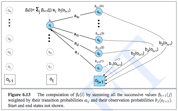
To estimate the parameters of the transition probability matrix, for a given element \(P(x_t \mid x_{t-1})\), we must count the expected proportion of times that the system undergoes a transition from state realization \(x_{t-1}\) to state realization \(x_t\). The expected counts are what EM computes, since those are the latent variables.

The following diagram shows the various things we have to compute to get the expected counts. Notice that the diagram is computing the probability of being in state \(i\) then state \(j\), jointly with the observation sequence. Thus, after this step, we would divide by \(P(e_{1:t})\) (or \(P(O \mid \lambda)\) in their notation). We then sum over all times, and that gives us the expected number of transitions from state \(i\) to state \(j\).

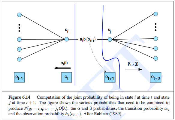
We follow a similar procedure for estimating the parameters of the emission probability.

The M-step is simple here; it turns expected counts into MLE for the corresponding parameters.

Particle Filtering

I got confused about particle filtering earlier. I assumed it broadly meant any algorithm that sampled something, but in fact, it has a specific meaning in the context of HMMs and Dynamic Bayesian Networks more generally. It is indeed a sampling algorithm, but has some interesting properties that are worth discussing in its own right.

First, when do we want to do particle filtering? We want to do this if exact inference in HMMs is intractable, or if the speed of sampling (and computing its corresponding probabilities) is more important than exact answers.

A naive way of performing exact inference in an HMM is to “unroll” it into a normal Bayesian Network. Technically, HMMs are infinitely long, so what we would do is chop off the HMM after the last time step that has a query or evidence variable, since by the structure of an HMM, anything after is not relevant to the query³. But if we did filtering after each observation, we would have to redo a lot of computations from the start \(X_0\) to the set of variables at the current time step. To save on memory costs, we realize that if we do filtering for a given time \(t+1\), we only need the relevant probability distribution from the previous time \(t\), since the computation is done recursively. Unfortunately, when we do this “summing out” process a-la variable elimination, that will iterate through the set of states, and this computation will grow exponentially due to the need to construct an exponentially large factor table⁴.

Thus, we need to use approximate inference methods. In a previous post, I discussed likelihood weighting, which is a sampling algorithm that we can adapt for the HMM setting. We do, however, have to ensure that we do not unroll the entire HMM, and we have to make sure our weights are not being driven to zero.

Likelihood weighting (just like rejection sampling) suffers as the number of evidence variables increases, because the weight of each sample is based on the product of all the \(P(E_i = e_i \mid E_{\pi_i})\) terms, which drives our values down to zero. But there is something that might be even worse than that. When we sample our non-evidence variables, ideally we would like those samples to depend on the evidence variables, so they can “guide” the sampling correctly. Unfortunately, if all the evidence variables tend to be downstream, i.e., they occur late in the variable ordering, then the sampling for the non-evidence variables will not depend on the evidence, even though the actual variables should depend on each other⁵. Sadly, in an HMM, all state variables have the property such that all the evidence relevant to them is downstream! (The ones before it are not downstream, but they are not ancestors either!)

What does particle filtering do, then, keeping in mind the weaknesses of likelihood weighting? Here is how the algorithm works. We initialize a population of \(N\) samples. The quantity \(N\) determines the time complexity of the algorithm, not the number of states. Then for each time step, we perform the following steps in sequence:

• We transition the samples according to the transition probabilities \(P(X_t \mid X_{t-1})\). This means we do not have to unroll the HMM.
• We then observe the evidence and downscale (i.e., multiply by a value in \([0,1]\)) each sample according to the evidence \(P(E_t \mid X_t)\). This is where the likelihood weighting “adaption” is obvious because now each sample is a fraction of a sample with some weight, and the overall distribution over the state variable’s realizations is the fraction of weights there divided by the total fraction of weights across all realizations.
• Then (and this is important), we resample to renormalize the distribution, where the resampling process is sampled according to the weights of the samples.

Here is a nice diagram from the CS 188 slides that suddenly clarified particle filtering for me.

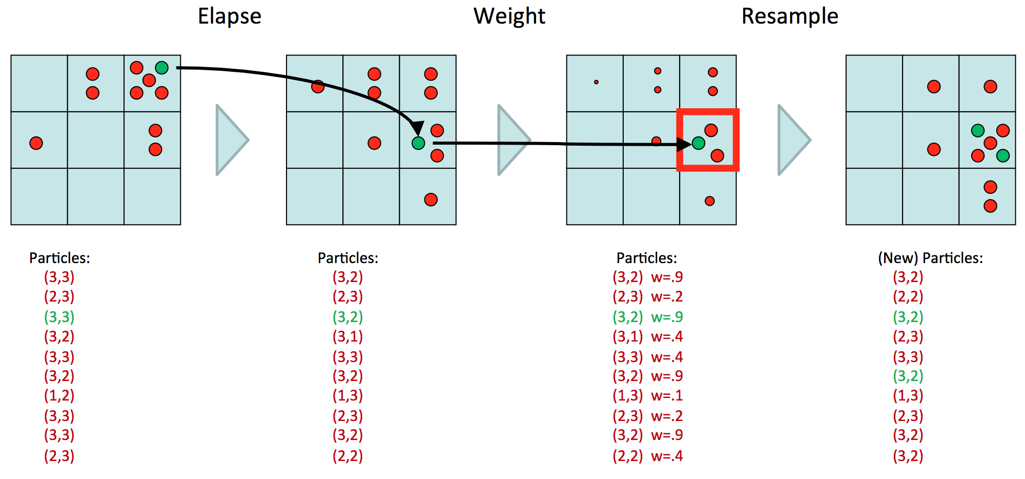
Here, we assume we have one state variable, with nine possible realizations. (Or we could have two state variables, each with three realizations, etc.) We have ten particles, representing our estimate of the distribution \(P(X_t \mid E_{1:t})\). Now the goal will be to determine the table of \(P(X_{t+1} \mid E_{1:t+1})\) values. First, we transition, which means we move each of the ten particles over to their next realization and multiply accordingly. Then, we observe \(E_{t+1} = e_{t+1}\), and downscale the values, resulting in points of different sizes, which are a diagram notation for weights. Above, we assume that whatever \(e_{t+1}\) was, the \(P(e_{t+1} \mid X_t)\) probability is high for that spot at coordinate \((3,2)\), and lower as we gradually go away from that spot. The last step is to resample, so we are resampling based on the probability distribution of the weighted samples. So we get five samples in that \((3,2)\) block because \(3(.9)\) divided by the sum of the weights (note: there’s a typo on the slides) gives a “high” probability. Note now that we have “normal-sized” samples again.

At this point, we should ask ourselves why we even bother resampling. It’s not completely clear to me, but it has to do with how we constantly rescale the weights downwards. In general, it’s not a good idea to have such small weights, because then the more evidence we have, the more likely we will just have a bunch of zero-probability particles. In other words, most particles end up in low-likelihood places in the state space. Still, I don’t quite buy some of the textbook explanations on this because couldn’t we just perform the computations in log space?

---

All right, I lied in the title of my last post. That wasn’t the final word on graphical models after all¹. In this post, we’ll discuss Expectation-Maximization, which is an incredibly useful and widespread algorithm in machine learning, though many in the field view it as “hacking” due to its lack of statistical guarantees². At first, I wasn’t sure what this had to do with graphical models. True, it’s not what I’d call core graphical models, but what happens is that a lot of problems that “factor” into nice Bayesian Network representations can use Expectation Maximization to determine the optimal value of their parameters (which are CPTs in the Bayesian Network case).

The Formalities of Expectation-Maximization

Expectation-Maximization (EM) is an extremely useful algorithm that applies in cases when we have a model with unobserved (i.e., latent) variables, and we need to train the model parameters despite the lack of that information. Why do we want latent variables? It helps to simplify our models. The canonical example is seeing a bunch of health measurements, then adding in a hidden node that represents the presence of heart disease.

We apply EM when we have some probabilistic model \(p(X,Z\mid \theta)\) in which we are trying to find the “best” model parameters \(\theta\), which usually means taking the Maximum Likelihood Estimate (MLE). Crucially, \(X\) is our observed variable (or a set of them), while \(Z\) represents the latent variables. Usually, we use logs when maximizing likelihood, so this is equivalent to finding \(\arg \max_\theta \log \sum_Z p(X,Z\mid \theta)\), which Mike calls the incomplete log likelihood³. This is hard; marginalization here (because it involves summing over \(Z\)) tends to “make problems harder.” My intuition: having sums means we don’t usually have a closed-form expression of the likelihood function, so how can we find the MLE for \(\theta\)?

We can define the expected complete log likelihood with some other distribution \(q(Z\mid X)\) as \(\sum_Z q(Z\mid X)\log p(X,Z\mid \theta)\), in other words, averaging out \(Z\). A good choice of \(q\) means that the expected log likelihood can be treated as the actual log likelihood.

EM is divided into two steps that repeat. Informally, the Expectation step assigns values to the hidden variables based on \(P(Z \mid X, \theta)\). (In most examples, these are indicator variables.) In the Maximization step, we find the MLE of \(\theta\), which is easy this time because we actually “know” what the \(Z\) variables are — we assigned them in the previous step!

There are two “formal perspectives” of EM, one relating to log likelihood, and the other relating to a concept known as the Kullback-Leibler Divergence.

The Log Likelihood View

Let us define the following quantity:

\[\mathcal{L}(q,\theta) = \sum_Z q(Z\mid X) \log \frac{p(X,Z\mid \theta)}{q(Z\mid X)}\]

We further know from some algebra that \(\mathcal{L}(q,\theta) \le \log \sum_Z p(X,Z\mid \theta)\), i.e., that \(\mathcal{L}\) defines a lower bound of the incomplete log likelihood, for an arbitrary \(q\) function.

We can now define our E and M steps more precisely:

• E step: \(q^{(t+1)} = \arg \max_q \mathcal{L}(p,\theta^{(t)})\)
• M step: \(\theta^{(t+1)} = \arg \max_\theta \mathcal{L}(p^{(t+1)},\theta)\)

What does this really mean? Note that in both cases we are trying to maximize a lower bound on the incomplete log likelihood, which makes intuitive sense: that is the point of MLE!

• In the E step, we are finding the best \(q\), and this can actually be solved analytically. It’s right under our noses: \(q^{(t+1)}(Z\mid X) = p(Z\mid X,\theta^{(t)})\). I mean, that’s just the true distribution of the hidden variable, given the known data and the current parameters! It sounds obvious.

  There are two ways to show this. One is to plug in that choice of \(q\) in the function \(\mathcal{L}(p,\theta^{(t)})\), and we get equality with the incomplete log likelihood, \(\log p(X\mid \theta)\). Hence, that’s the best \(q\) we can get! The other is to take the KL-Divergence view (spoiler for the next section!) and see that

  \[\log p(X\mid \theta) - \mathcal{L}(q,\theta) = KL(q(Z\mid X)\: \| \: p(Z\mid X,\theta))\]

  which shows that to minimize the difference between the two distributions, we need to set the two distributions to be the same. Remember again that \(\mathcal{L}\) is a lower bound. I know I say this a lot, but it’s important.

• In the M step, we maximize the expected complete log likelihood, which we recall we defined earlier as \(\sum_Z q(Z\mid X)\log p(X,Z\mid \theta)\). This happens because \(\mathcal{L}(p,\theta)\) breaks into two terms, one which is the expected complete log likelihood, and the other which does not depend on \(\theta\).

Taken together, what do these steps really do? Let’s look back at the incomplete log likelihood \(\log p(X\mid \theta)\). This is hard to optimize, as we said earlier, but what the E and M steps do is that, during each iteration, they collectively keep maximizing this function! It’s a “hill climbing” algorithm that will keep increasing (or technically, never decrease) the incomplete log likelihood. Why is that the case? Here’s the intuition. The M step means that we are maximizing \(\mathcal{L}(q,\theta)\), a lower bound to the incomplete log likelihood. Hypothetically, suppose \(\mathcal{L}(q,\theta)\) was actually equal to that incomplete log likelihood. Then the M step would necessarily result in a (highly desirable!) increase in \(\log p(X\mid \theta)\). But this only works if there is equality … if there is a gap, the plan is thrown out the window.

Fortunately, the E step comes to rescue us, because we already know that for an appropriate choice of \(p\), we can get \(\mathcal{L}(p,\theta)\) to be equal to \(\log p(X\mid \theta)\). Note that the thetas here should really have a time superscript attached to them (as well as the \(p\)s) but I left them out for simplicity.

In conclusion, EM will keep increasing \(\log p(X\mid \theta)\) each iteration. This, if you recall, was the whole point of this process anyway! And it does this by cleverly optimizing the \(\mathcal{L}(q,\theta)\) function, which is much easier to handle than the incomplete log likelihood. Absolutely brilliant!

The Kullback-Leibler Divergence View

We can alternatively bound the KL-Divergence. Derive the bound

\[KL(\tilde{p}(X) \: \| \: p(X\mid \theta)) \le KL(\tilde{p}(X)q(Z\mid X) \: \| \: p(X,Z\mid \theta))\]

In words: the KL-divergence between the empirical distribution \(\tilde{p}(X)\) and the model \(p(X\mid \theta)\) is upper bounded by a “complete” KL-divergence. The intuition is that we are adding in the \(q(Z\mid X)\) to “average over” the values of \(Z\), just as we did earlier with the expected complete log likelihood term.

Our results carry over from the previous section because minimizing the right hand side of that expression above (with respect to \(q\) and \(\theta\)) is equivalent to maximizing \(\mathcal{L}(p,\theta)\) with respect to the same variables. Why? As part of the derivation for that bound above, we invoked \(\log p(X\mid \theta) \ge \mathcal{L}(p,\theta)\), but that part was embedded inside an expression such that there was a negation attached, so maximizing \(\mathcal{L}\) means minimizing the overall problem.

Letting \(KL(q\: \|\: \theta) = KL(\tilde{p}(X)q(Z\mid X)\: \| \: p(X,Z\mid \theta))\), the steps are:

• E step: \(q^{(t+1)} = \arg \min_q KL(q\: \| \: \theta^{(t)})\)

• M step: \(\theta^{(t+1)} = \arg \min_\theta KL(q^{(t+1)}\: \| \: \theta)\)

Example on Gaussians

This example is from Russell and Norvig (2010). It is about clustering on a dataset presumed to be generated by three unknown multivariate Gaussian distributions. Here’s an example of a plot that could represent such data, with each data point highlighted by the color of its distribution (which we would not know — they are only there for ease of readability). Note: the figure here isn’t the exact one in the textbook, but it’s close.

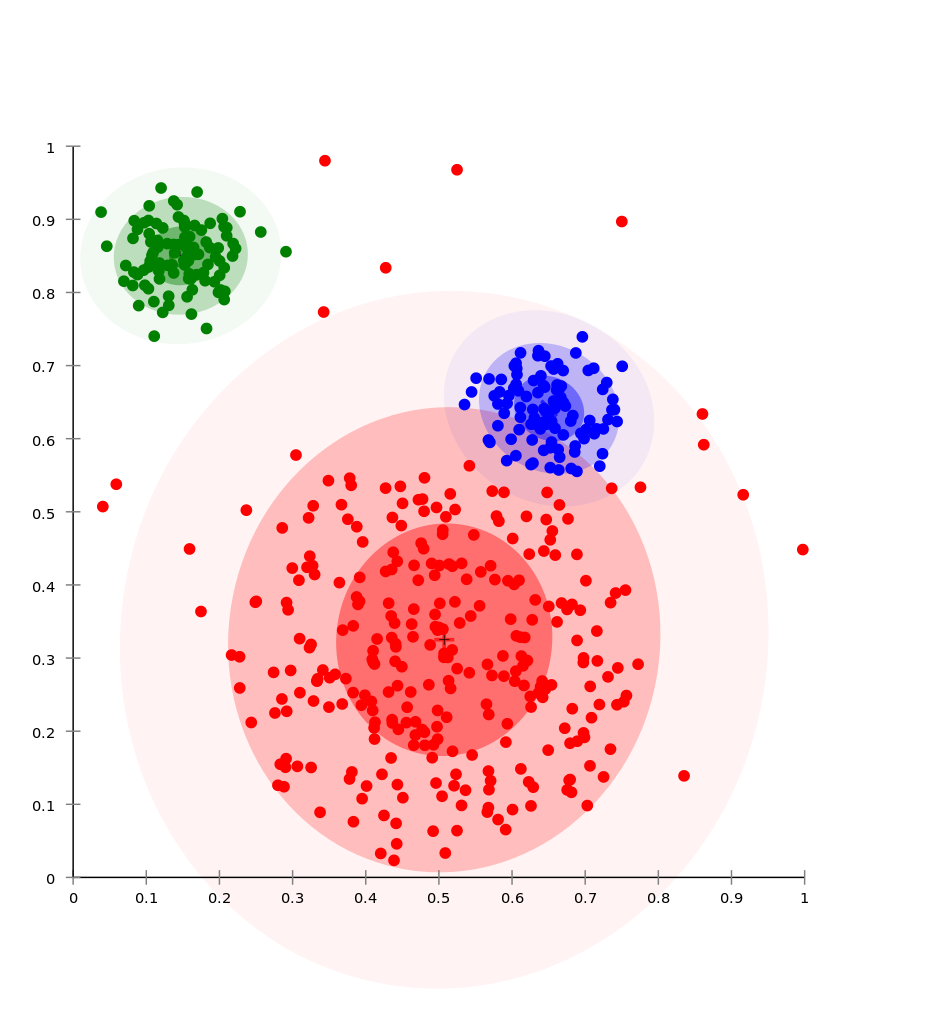
I like this example because it makes it clear how to view the \(Z\)s as indicator variables.

To formalize the problem, we assume that each data point is generated by picking one of the three two-dimensional, multivariate Gaussian distributions, then sampling from that distribution. Thus, the goal in using EM is to find the parameters of the model:

• the weight \(w_i = P(C = i)\) of each component (i.e., each multivariate Gaussian)
• the 2-dimensional mean vector \(\mu_i\) of each component
• the \(2\times 2\) covariance matrix \(\Sigma_i\) of each component

To start off with EM, we first initialize the three sets of parameters above to some random values⁴. Then we iterate:

• E step: this will determine the expected value of the hidden indicator variables in this model, which we define as \(Z_{ij}\), which is one if point \(x_j\) was generated by Gaussian component \(i\) and zero otherwise. From the earlier discussion, we know that we need to use the \(p(Z\mid X,\theta)\) function. Assuming that the points are IID, this means for each point \(x_j\), we compute \(\mathbb{E}[Z_{ij}] = p(Z_{ij}=1 \mid x_j,\theta^{(t)})\) where \(i \in \{1,2,3\}\).

  We can transform this into an easier problem using Bayes’ rule, and claim that \(p(Z_{ij} = 1 \mid x_j,\theta^{(t)}) \propto p(x_j \mid Z_{ij}=1,\theta^{(t)})p(Z_{ij} = 1\mid \theta^{(t)})\). The first quantity, \(p(x_j \mid Z_{ij}=1,\theta^{(t)})\), is a straightforward plug and chug into the formula for the density of a multivariate Gaussian, because we assume it came from the \(i\)th one, and we have the parameters \(\mu_i\) and \(\Sigma_i\) from \(\theta^{(t)}\). The second quantity, \(p(Z_{ij}=1 \mid \theta^{(t)})\) is like computing the probability that a component generated a given point, but without any dependency on any point \(j\), we just probabilistically choose based on the component’s overall weight \(w_i\), which we get from \(\theta^{(t)}\).

• M step: given the fact that we “know” which component \(i\) generated which data point \(x_j\) in a probabilistic sense, then we can find better values of the parameters using the following update equations:

  • The weights: \(w_i \leftarrow n_i/N\)
  • The means: \(\mu_i \leftarrow \sum_j \mathbb{E}[Z_{ij}]x_j/n_i\)
  • The covariances: \(\Sigma_i \leftarrow \sum_{j} \mathbb{E}[Z_{ij}](x_j - \mu_i)(x_j - \mu_i)^\top/n_i\)

  where \(N\) is the total number of data points and \(n_i = \sum_j \mathbb{E}[Z_{ij}]\), the “number” of data points assigned to component \(i\) (in a probabilistic sense).

  Why does the M step work? The weight update is like that because that is the fraction of points we assigned to that cluster, and \(\sum_i \sum_j \mathbb{E}[Z_{ij}] = N\). The means and covariances is from the MLE for the parameters of multivariate Gaussians, except that we have to scale by an expectation because clusters are only assigned fractions of points.

For a more complicated example of EM, look at how EM is used to train the parameters of Hidden Markov Models.

---

The Basics

There are two main types of graphical models: directed (Bayesian Networks) and undirected (Markov Random Fields). There are also chain graphs that mix the two, but I will ignore those for now. Bayesian Networks are interesting because they let us model generative processes. We can look at arrows in a diagram and think: oh, there’s an arrow from \(X_1\) to \(X_2\), hence the former variable must have some kind of causal relationship with the latter. Then we can continue that line of thinking to “generate” each variable. For a Markov Random Field, we can think of there being a local structure to the nodes.

One of the main reasons why people like graphical models is that it helps us concisely express probability distributions. If we have a distribution \(P(X_1,X_2,\ldots,X_n)\) where \(n\) is in the hundreds (a typical real-world case) a naive tabular representation of the distribution is out. But with a Bayesian Network, what we can do is decompose the joint into node-parent conditional probability tables (CPTs). Using the chain rule on a Bayesian Network, with nodes listed in a topological ordering¹, we can decompose the joint into distributions of each node, and then use the independence assumption to get rid of (hopefully lots of!) certain variables being conditioned on in \(P(X_i \mid X_1, X_2, \ldots, X_{i-1})\). For a Markov Random Field, we can decompose the joint probability into a product of functions on maximal cliques, \(P(X_1,\ldots,X_n) \propto \prod_{X_C \in \mathcal{C}} \psi_C(X_C)\), where \(\mathcal{C}\) is the set of maximal cliques of the graph². One of the most confusing things about the clique functions \(\psi\) is that they are not (generally) probability distributions! All we require is that they are an arbitrary, local non-negative function. To enforce non-negativity, it is common to exponentiate functions, thus we often see these expressed in terms of exponentials³. Note: it’s important to understand the high-level idea here. In both the directed and undirected cases, we have figured out a way to efficiently decompose the joint into the product of functions that act on a local set of nodes.

Given that we have decomposed the joint distribution in terms of products of local functions, it’s important to realize that, while we’ve obviously imposed some “constraints” on the graph, a graphical model still expresses a family of distributions. In a three-node “chain” Bayesian Network, which means \(P(X_1,X_2,X_3) = P(X_1)P(X_2\mid X_1)P(X_3\mid X_2)\), we are allowed to tweak the three CPTs of our graph, so long as the product still obeys a probability distribution (i.e., non-negative and sums to one). For a Markov Random Field, we can tweak the potentials.

There is also an equivalent way of expressing the family of distributions inherent in a graphical model. We can do that by listing all the conditional independences enforced by the graph. This means that for all triplets of disjoint variable sets \(X_A,X_B,X_C\) which are a subset of all the variables in the graph, we need to check whether \(X_A \perp X_B \mid X_C\). By taking the set of distributions that factor according to these independences, we find that they are equivalent to what we would get if we started with the node-parent probabilities and “tweaked the CPTs.”

It’s easiest to determine whether \(X_A \perp X_B \mid X_C\) in the undirected case, because to determine whether such a statement is true (and therefore should be listed in that list of independences) we delete the nodes of \(X_C\) and check whether a path still exists from \(X_A\) to \(X_B\).

The directed case is a little more complicated, but more intellectual. We run something called the Bayes Ball algorithm. To explain this, we first consider three canonical graphs: a chain \(A \rightarrow B \rightarrow C\), a wedge \(A \leftarrow B \rightarrow C\), and (the most interesting case) a v-node \(A \rightarrow B \leftarrow C\). The rules are as follows:

• In the chain, \(A \perp C \mid B\). No other assertions are possible.
• In the wedge, \(A \perp C \mid B\). No other assertions are possible.
• In the v-node, \(A \perp B\). No other assertions are possible.

To explain the third case in more detail is to understand the explaining away phenomenon. This happens when we have two or more competing clauses that attempt to explain the same thing. Those clauses are independent of each other, but once we observe the \(C\) variable, then all of a sudden they are dependent on each other, because if one of them “caused” \(C\), it is likely that the other one did not. But without \(C\), we can’t say much. Kevin Murphy has a nice example on his tutorial page, where a college only admits smart students, or athletes, and those variables are independent in the population. Then if we see that a student is at the college, then we can “explain” this phenomenon in two ways: if the student is smart, or an athlete.

To run the Bayes Ball algorithm, we “shade in” the nodes of \(X_C\), which serve intuitively as “blocking” nodes. We start with balls in nodes from \(X_A\), and see if any one of them can reach any node in \(X_B\), subject to constraints on the movements of the balls due to the canonical graphs. Note that there are a few other special cases that we have to consider. If we have a chain \(A \rightarrow B\) but \(B\) has no other children, then the ball is allowed to “return” in the opposite direction, so long as \(B\) is shaded. It is as if there is a duplicate \(A\) node, which would be like applying case three with the v-node, and balls only pass in that case if the \(B\) node is shaded.

So, if you are ever given a Bayesian Network and have to determine whether certain conditional independences hold, just as in the Spring 2011 Berkeley AI final, just run the Bayes Ball algorithm.

By the way, it should be clear from the above that identifying conditional independences is easier for the undirected case, which is what tends to motivate their formulation, but for the directed case, it’s easier to think of them in terms of node-parent probabilities. But we could try thinking of them in the opposite way.

The Sum-Product Algorithm and Factor Graphs

In my last post, I described two ways of performing exact inference on general graphical models. That’s actually not the final word on exact inference: it is possible to develop a more useful version of variable elimination, under the assumption that the graphical model is a tree. This is not that restrictive, since we can express a lot of real-world problems in terms of trees. The key advantage of the algorithm known as the Sum-Product Algorithm⁴ is that it lets us compute all marginals simultaneously. If you recall, in variable elimination, I assumed that we only had one query node, so that algorithm would have been useful for \(P(X_i \mid e)\), but not \(P(X_i,X_j \mid e)\). Fortunately, with trees, we can compute all of \(P(X_i)\) for each node. Including evidence isn’t a problem; we can also compute \(P(X_i,e)\). Remember that we should consider marginals and conditionals as equivalent.

How does it work? Remember how in variable elimination, we would create intermediate values \(m_i(...)\) for node \(X_i\) as it got eliminated? We will do a similar thing here; these \(m_i\) are now technically called messages and we can index them as \(m_{ij}(...)\) to describe a message from node \(X_i\) to \(X_j\), where node \(X_i\) was the one that got eliminated.

The Sum-Product algorithm begins message-passing at the leaf nodes of the graph by eliminating them and passing their intermediate messages (the \(m_i\) functions) to their neighbors. Then the process repeats. The rule is that each node can only send a message to another node, as long as it has received messages from all its other neighbors. Since the graph is a tree, this immediately implies that messages have to start at the leaves (as stated earlier) and, furthermore, that no new edges will be created in the elimination process.

To be precise, the formula for a message from \(X_j\) to \(X_i\) (hence, eliminating \(X_j\)) is:

\[m_{ji}(x_i) = \sum_{x_j} \psi^E(x_j) \psi(x_i,x_j) \prod_{k \in \mathcal{N}(j)\setminus i} m_{kj}(x_j)\]

This equation is from Michael I. Jordan’s notes on graphical models. Don’t worry too much about the notation, but here is a little about it: the \(\psi^E\) function is his way of including evidence variables⁵. The \(\psi(x_i,x_j)\) is the potential function on the maximal clique of \(X_i\) and \(X_j\); in trees, the maximal cliques are always of size two. The interesting stuff comes when we consider the \(m_{kj}\) functions. These are all the other incoming messages from the neighbors of node \(X_j\), except \(X_i\). This should remind us of variable elimination. When we eliminate nodes, we pass intermediate factors back to whatever node has dependency on it. Since we are in a tree, that means the intermediate message will have a dependency on whatever neighbor is remaining. That is why the \(m_{kj}\) functions depend on \(x_j\), but the \(m_{ji}\) function depends on \(x_i\) (not \(x_j\)).

Oh, by the way, we are dealing with undirected graphs here, not directed ones. We can treat these on equal footing because we have trees, so in the undirected case, \(\psi(x_i,x_j) = P(x_j \mid x_i)\), and the singleton potentials are either 1, or \(P(x_r)\) for the root⁶.

At the root node, we can determine the marginal probability as proportional to the product of incoming messages, where the proportionality can be resolved by iterating over the possible states/realizations for the root node.

That’s nice, but how do we determine marginal probabilities for all nodes? When we did this for the root node, it was as if the messages started from the leaf nodes and propagated inwards towards the root node, due to the protocol that a node couldn’t send a message unless it got messages from all other neighbors. The clever insight is that we now propagate messages outwards from the root node, into all the leaves! What happens after this is that every edge in the tree now has two messages on it, in opposite directions. Then, for each node, take the product of its incoming messages. We now have marginal probabilities for all nodes! The amazing thing is that this only requires double the amount of work it took for the first step to send messages inwards to the root. Unfortunately, as mentioned earlier, this only works on trees. But it definitely works well.

Taking another perspective, suppose we were not interested in determining a distribution, but wanted to do MAP inference. That means figuring out the maximum probability possible in any configuration (or determining the actual configuration itself). To do that, just replace the “sum” operators with “max” operators in the formulas, and things will work from there⁷.

Finally, let us consider factor graphs, briefly. Given an undirected graph, we can associate with it a set of factors \(\mathcal{F}\), where each factor \(f_i(X_{f_i})\) is a function on a set of nodes. The sets may not be unique among different factor functions, and they might not also correspond to maximal cliques. Actually, the one thing we really want them to obey is that there is a giant factor function \(f\) of all the variables that can be “factorized” (hence the name) into the individual factors, and that we can evaluate for one factor efficiently (kind of reminds one of probabilities and potentials, huh?). Then when we draw the graph, the only edges that exist are those from normal nodes \(X_j\) to factor nodes \(f_i\), and an edge exists between them if and only if the factor function \(f_i\) takes node \(X_j\) as input.

Some advantages of factor graphs are that:

• Sometimes, we want to express a family of probability distributions at a finer level than is possible with conditional independences. Factor functions let us be arbitrarily precise in how we want to model the interactions between variables, while potential functions are more limited. With the complete graph \(\mathcal{K}_3\), no conditional independence assertions are possible but we might want to endow the sole potential with some structure: \(\psi(x_1,x_2,x_3) = f_a(x_1,x_2)f_b(x_2,x_3)\), but note that adding extra nodes can do the same thing⁸.
• We can convert undirected trees that are “almost” like trees (perhaps they have just one clique of size three) into factor graphs that are trees, ignoring the distinction between factor and variable nodes.
• We can apply a similar version of the sum-product algorithm to factor trees, which uses messages from nodes to factors and factors to nodes, even if the original tree (before the factorization was added) was not actually a tree.

There are also directed graphs that are almost like trees, e.g., polytrees, which are trees if we drop the orientation of edges, but they also have multiple parents to each node, which poses a problem if we do any moralization. We can convert these to factor trees (yes, trees) and directly apply the Sum-Product algorithm.

Sampling for Graphical Models

In many cases, exact inference is intractable in graphical models, so we resort to approximate methods. Here, I’ll briefly review approximate inference in Bayesian Networks, with an emphasis on particle-based methods, which generate samples from the network.

One confusion I originally had when I first learned about this was that it was unclear what assumptions we were making about the information we possessed. To clarify, we’re going to assume that we know all the CPTs⁹ of the graph, but that’s it. The goal will be to generate a full set of samples from this CPT. That means if there are \(n\) variables in the Bayesian Network, we want to obtain samples \((X_1,X_2,\ldots,X_n)^{(i)}\) for large \(i\).

Using the CPTs, how do we sample? Here’s an almost trivial method, often called direct sampling: we iterate through the variables in a topological ordering, and for each one, sample its state¹⁰ from its CPT. The parents of the node in question (if any) must be set to the value that they were sampled at earlier, which we know happened due to the topological ordering. Once we’ve gone through all samples, we repeat.

In the general case, we’ll want to make use of whatever evidence variables we have in \(P(X \mid E = e)\), which direct sampling fails to consider. To do so, we can use rejection sampling, which means that we do direct sampling, but only keep the full samples that are consistent with the evidence \(E = e\). Unfortunately, as the evidence increases, it gets increasingly unlikely that we will ever generate a compatible sample! To fix the problem of rejecting too many samples, we can use likelihood weighting which will force the evidence variables to be at their fixed values. That is to say, given a network of \(n\) variables where we want to sample full elements that have \(X_i = 2\), then we would fix that value and sample the other \(n-1\) variables normally with the direct sampling method.

Unfortunately, even this doesn’t work out well, because we actually have to weigh the samples we get by the value of the evidence variables! It’s easiest to think of likelihood weighting as always generating compatible samples, but each sample is actually worth only a fraction of a sample, quantified by its weight \(w\). We compute a sample’s weight by multiplying the \(P(X_i = x_i \mid X_{\pi_i})\) values of the evidence variables together. Intuitively, evidence variables that seem to be incompatible with the sampled variables should result in a smaller weight for the full sample.

Rejection sampling and likelihood weighting are two valid sampling methods, but they generate full samples independently of each other. The class of Markov Chain Monte Carlo methods assume that consecutive, full samples are (weakly) correlated with each other. Gibbs Sampling is the most well known of these samples. Given \((X_1,X_2,\ldots,X_n)^{(i)}\), it goes through each variable one by one and generates a sample for variable \(X_j\) in the \((i+1)\)th element by using the conditional distribution

\[P(X_j^{(i+1)} \mid X_1^{(i+1)}, \ldots, X_{j-1}^{(i+1)}, X_{j+1}^{(i)}, \ldots, X_{n}^{(i)})\]

Thus, it relies on the newly generate samples for the first \(j-1\) variables, but for the remaining variables, it uses the values of the previous sample. Hence the correlation between consecutive samples.

But wait, in a Bayesian Network, we can say more! The probability of a variable, conditioned on all the other variables, is simply that conditioned on the Markov blanket of a variable, which consists of itself, its parents, its children, and the parents of those children! We need to make an important distinction: when we say that \(P(X_i \mid X_1, \ldots, X_{i-1}) = P(X_i \mid X_{\pi_i})\) in Bayesian Networks, that is only because we list variables in a topological ordering. If the variable is conditioned on all other variables in the network, we can only simplify by eliminating variables that are outside the Markov blanket \(mb(X_j)\) of a node. Precisely, Gibbs sampling would sample from the following distribution:

\[P(X_j \mid mb(X_j)) \propto P(X_j \mid X_{\pi_j}) \prod_{Y_j \in C(X_j)} P(Y_j \mid Y_{\pi_j}),\]

where \(C(X_j)\) denotes the set of children nodes of node \(j\).

Note: with evidence variables, we just don’t sample them in Gibbs sampling (which also applies to other sampling methods).

Putting all this together, what does it really mean when we generate full samples? How do these actually help us with a query? An example would clarify. If we are making the query \(P(X_1 \mid X_2 = x_2, X_3 = x_2)\), but this is not a node-parent probability (i.e., it is not listed in the CPTs anywhere) we need to sample to figure out the distribution of \(X_1\). Thus, we would generate full samples. We can then compute the desired distribution by looking at the value of \(X_1\) generated in all those samples that have \(X_2 = x_2\) and \(X_3 = x_3\) (i.e., that are consistent). In other words, it’s a maximum likelihood estimate.

What I Would Study Next

If I had all the time in the world to study graphical models, here’s what I would study next: the junction tree algorithm. This is an extension of variable elimination and the sum-product algorithm in that it performs exact inference on general graphical models as efficiently as possible. To do that, it has to transform the graph into what’s known as a junction tree (hence the algorithm name). Unfortunately, that’s about all I know about the algorithm.

---

In an effort to help me understand certain topics better for my prelim exam next month, I thought I’d briefly write about a topic that I sometimes never feel like I understand completely: exact inference in graphical models. Given a graphical model, inference is simply the task of computing the probability $P(X = x \mid E = e)$, where \(X\) is a set of query variables, \(E\) is a set of evidence variables, and if we include another disjoint set \(H\) of the hidden variables, then \(X \cup E \cup H\) represents the entire set of nodes in the graphical model. In general, inference is intractable, but for now we’ll pretend not to worry about that by discussing two ways of doing exact inference: by enumeration, and by variable elimination.

Inference by Enumeration

Here’s an example of a Bayesian Network, i.e., a directed graphical model with seven variables. This comes from the spring 2011 final for Berkeley’s undergraduate AI course, and the reason why there’s one \(Y\) but six \(X_i\)s is because the question using this graphical model wanted to emphasize how the \(Y\) represented a class variable. But it’s still a variable, just like all the $X_i$s, so the distinction is not important now.

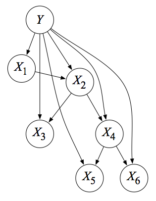
Suppose we want to compute the exact quantity of¹ \(P(X_2 = x_2 \mid X_4 = x_2)\). The first key point we need to know is that this computation immediately reduces to the computation of the joint \(P(X_2 = x_2, X_4 = x_4)\), which directly follows from the definition of the conditional probability. Once we compute that joint, we can then divide by \(P(X_4 = x_4)\). Or, better yet, since the denominator does not depend on the value we choose for \(X_2\), we can avoid computing it by determining \(P(X_2, X_4=x_4)\) while substituting in the possible states of \(x_2\). These values will give us the normalizing constant we need, because we will be computing a vector of probabilities (one element per assignment to \(X_2\)) and the normalizing constant is the sum of all those elements. The point of all this previous discussion is this: the computation of conditional probabilities immediately reduces to the computation of joint probabilities.

Joint probabilities are easier for me to digest. In the current example, the joint can be re-expressed (using the simpler form of omitting the capital variables) as

\[\begin{align} P(x_2, x_4) &= \sum_y \sum_{x_1} \sum_{x_3} \sum_{x_5} \sum_{x_6} P(y, x_1, x_2, x_3, x_4, x_5, x_6) \\ &= \sum_y \sum_{x_1} \sum_{x_3} \sum_{x_5} \sum_{x_6} P(y)P(x_1\mid y)P(x_2\mid x_1,y)P(x_3\mid x_2,y)P(x_4\mid x_2,y)P(x_5\mid x_4,y)P(x_6\mid x_4,y) \\ &= \sum_y P(y)P(x_4\mid x_2,y) \sum_{x_1} P(x_1\mid y)P(x_2\mid x_1,y) \sum_{x_3} P(x_3\mid x_2,y) \sum_{x_5} P(x_5\mid x_4,y) \sum_{x_6} P(x_6\mid x_4,y). \end{align}\]

Notice that we split up the joint into the conditionals described by the network, and then pushed the summations as far right as possible. The notation \(\sum_y P(y)\) means that if \(Y \in \{1,2,3\}\), we are determining \(P(Y=1)+P(Y=2)+P(Y=3)\), i.e., we sum over the possible states of \(Y\). So, in the above algebra, we sum over the possible set of states for the variables other than \(X_2\) and \(X_4\), which are assumed fixed, but we still denote their values \(x_2\) and \(x_4\) with lowercase variables. Sorry. As my former professor Ben Recht would say, “the worst part about this is the notation.”

We need to be careful to make sure that we are rearranging the sums and probabilities correctly. For instance, \(P(y)\) is all the way to the left because it only depends on \(Y\), but so is \(P(x_4\mid x_2,y)\)! The reason is, again, that \(X_4\) and \(X_2\) are fixed to those values, so there is no dependency over any other summation.

At this point, exact inference by enumeration simply means computing the quantity above from left to right. So we would first fix \(Y\) to a state, then compute \(P(y)P(x_4\mid x_2,y)\), then loop over the values for \(X_1\), and so on. It’s basically like how we have nested for loops in computer programming. This will give us the exact values. Then we have our desired conditional determined up to proportion: \(P(x_2\mid x_4) \propto P(x_2,x_4)\). To get the exact value, repeat the computation for all states of \(X_2\).

Variable Elimination

Variable elimination is the same as inference by enumeration, except for two things: (1) that we compute right to left and that (2) the exact order of our summations will change based on our variable ordering. That’s it! The key advantage of variable elimination over enumeration is that variable elimination is a dynamic programming algorithm and re-uses computation.

I’m not going to go through the entire variable elimination algebra here, because the notation is tedious and we will do an example later, but here would be the first step. In the math above, we would transform \(\sum_{x_6} P(x_6\mid x_4,y)\) into an intermediate factor \(m_6(y)\), where the subscript 6 denotes the variable we just eliminated, and \(y\) indicates the variable it depends on (it does not depend on the “variable” \(x_4\) because it is fixed, but we are still summing over values of \(Y\))². Then we repeat the process by creating more intermediate factors by going right to left. If we had to re-do a lot of computations in enumeration, then variable elimination will save us lots of computation time.

Some notes:

• It is possible to view variable elimination in a graph-theoretic way on undirected graphs. Here’s what happens: for a Markov Random Field, we use the graph directly, and for a Bayesian Network (like the one above), we would first moralize the graph by iterating through each node in the graph, connecting its parents, and then dropping the orientation of its edges. Great, so now we have an undirected graph – what now? First, we need a variable elimination ordering where the query variable (\(X_2\) in the above example) is listed last³. Then, for each variable in the ordering, we eliminate it. For a variable \(Z\), this means – graphically – that we would connect all neighbors of \(Z\) with an undirected edge (this forms a clique!), then eliminate \(Z\) from the graph. We repeat this process for all variables, until we get to our query variable, upon which time we will know the value of interest for the probability.

• The order in which we eliminate variables is crucially important. This is beyond the scope of this post, but the run time of variable elimination is dominated by the size of the largest clique formed in the graph-theoretic version I just described. This is formalized as the treewidth of the graph, which is defined as one less than the size of the largest clique formed, in the best possible variable ordering for the graph. Unfortunately, it is intractable to know the optimal variable ordering, but we can have heuristics.

I need to add a word of caution to the first bullet point above. There are different ways of interpreting variable elimination⁴. Some sources do not include the query variables in the elimination ordering, because it is assumed fixed (and it is always last so why bother). Similarly, some would also not include the evidence variables (\(x_4\) in our case) because we are not “eliminating” them. To me, it is a little unclear how this works graphically. What happens when we eliminate a variable that is connected to an evidence or query variable? Do we have to add edges between pairs of nodes where at least one is a query or evidence node? Do we eventually delete the evidence nodes? (We would never delete the query one because it is always last and by the time we finish, that node is the only thing left in the graph.) For now, my interpretation is that I’ll keep the query and evidence variables in the graph⁵. If we eliminate a neighbor, we just don’t add edges to those nodes, because there is no “interaction” with those variables – again, the query and evidence values are fixed. If we end up with no edges towards one of the evidence variables at any point in the query, then I guess we can finally remove the node. My definition of elimination means that we can only “eliminate” a variable that corresponds to one of the summations \(\sum_x\) in the above algebra.

Variable elimination – like inference by enumeration – takes exponential time in the worst case, based on the size of the conditional probability tables of the graphical model. In practice, as long as a graph of interest has a small enough treewidth (which usually means up to three), we can apply the algorithm. In a special class of graphs known as polytrees, inference takes (gasp) linear time!

With that said, we now turn to an example to apply our knowledge.

Example

Now let’s get back to that original question on the spring 2011 Berkeley AI final exam. I find practice exams (with solutions) to be among the gold mine for learning. Sometimes I learn more from practice finals than by reading an entire textbook! So it’s worth the time to go over the questions. The solutions key is already online, but for the variable elimination questions, I will go over the algebra and discuss the answers in more depth.

Here’s part (a):

Suppose we observe no variables as evidence in the TANB above. What is the classification rule for the TANB? Write the formula in terms of the CPTs (Conditional Probability Tables) and prior probabilities in the TANB

This isn’t really graphical-model related, because it’s simply \(\arg \max_y P(y)\). We could re-express \(P(y)\) with the other six variables if we have the patience to write out six \(\sum_x\)s.

Here’s part (b):

Assume we observe all the variables \(X_1 = x_1,X_2 = x_2,\ldots,X_6 = x_6\) in the TANB above. What is the classification rule for the TANB? Write the formula in terms of the CPTs and prior probabilities in the TANB.

Now we really do have to write things out explicitly, because the classification rule is \(\arg \max_y P(y,x_1,x_2,x_3,x_4,x_5,x_6)\), with all variables fixed (except for \(Y\), but we are fixing it here when we have to try different values of \(y\)). Here’s the joint I wrote earlier but will repeat here:

\(P(y)P(x_1\mid y)P(x_2\mid x_1,y)P(x_3\mid x_2,y)P(x_4\mid x_2,y)P(x_5\mid x_4,y)P(x_6\mid x_4,y)\).

We will have to use this joint in part (c), which finally introduces us to variable elimination:

Specify an elimination order that is efficient for the query \(P(Y \mid X_5 = x_5)\) in the TANB above (the query variable \(Y\) should not be included your ordering). How many variables are in the biggest factor (there may be more than one; if so, list only one of the largest) induced by variable elimination with your ordering? Which variables are they?

Now things get interesting. How do we determine an efficient variable elimination? The idea is that we come up with an ordering, then see the \(m_i(x_j,\ldots)\)s we get, and make sure that the largest \(m_i\) function is “not too large.”

A useful first step that I use is that, after moralizing the graph, I see if there is any variable I can eliminate that will not create any additional edges. First, I notice that the variables \(X_3\) and \(X_6\) both have the property that their parents are connected in the moralized graph. Thus, removing those two variables should not add new edges, and so the largest clique will remain small. The clique will be of size two, as we are not counting the evidence or query variables.

It then remains to determine an ordering for \(\{X_1,X_2,X_4\}\). For that, I would look at the moralized graph with edges removed or added (none added in this case so far), and then try and see if I could eliminate nodes that would involve creating as few new edges as possible. The following picture shows my drawing of the variable elimination, because it would have taken forever to typeset this in LaTeX using the tikz library. Spoiler alert: I’ve already done the full elimination. I will describe why it makes sense to do this shortly.

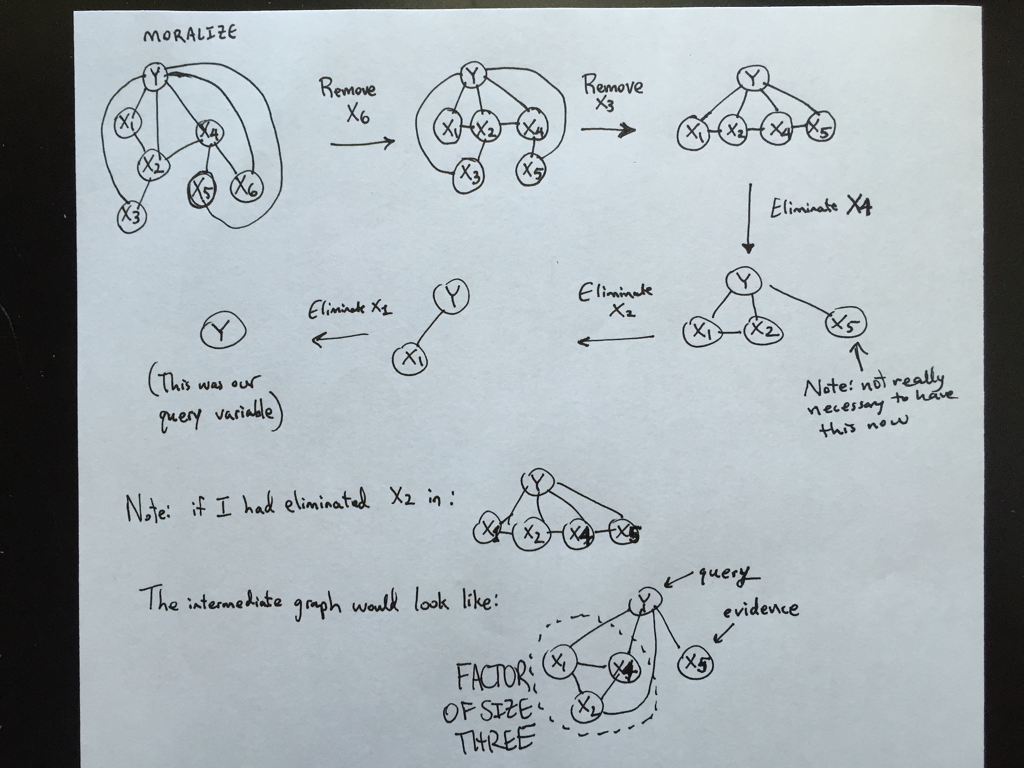
Algebraically, this corresponds to the following⁶, a right-to-left evaluation where we start with the full joint and then shift the summations and probabilities around:

\[\begin{align} P(Y=y \mid X_5=x_5) &\propto \sum_{x_1}\sum_{x_2}\sum_{x_3}\sum_{x_4}\sum_{x_6} P(y)P(x_1\mid y)P(x_2\mid x_1,y)P(x_3\mid x_2,y)P(x_4\mid x_2,y)P(x_5\mid x_4,y)P(x_6\mid x_4,y) \\ &= \sum_{x_1}\sum_{x_2}\sum_{x_4} P(y)P(x_1\mid y)P(x_2\mid x_1,y) P(x_4\mid x_2,y)P(x_5\mid x_4,y)\underbrace{\sum_{x_3} P(x_3\mid x_2,y)\underbrace{\sum_{x_6}P(x_6\mid x_4,y)}_{= 1}}_{= 1} \\ &= P(y) \sum_{x_1} P(x_1\mid y) \sum_{x_2} P(x_2\mid x_1,y) \underbrace{\sum_{x_4} P(x_4\mid x_2,y)P(x_5\mid x_4,y)}_{m_4(x_2)} \\ &= P(y) \sum_{x_1} P(x_1\mid y) \underbrace{\sum_{x_2} P(x_2\mid x_1,y) m_4(x_2)}_{m_2(x_1)} \\ &= P(y) \underbrace{\sum_{x_1} P(x_1\mid y)m_2(x_1)}_{m_1} = P(y)m_1. \end{align}\]

Notice that indeed, it makes sense to get rid of \(X_3\) and \(X_6\) since they are simple cases that sum away to one. In fact, the solutions manual says that these variables should not even be included in a variable elimination ordering.

Next, we have to consider some combination of \(X_1,X_2,\) and \(X_4\) to eliminate. The ordering here does matter! Here’s why: both \(X_1\) and \(X_4\) are connected to one other variable (\(X_2\)) and the two other nodes that represent fixed values. But \(X_2\) is connected to two other variables! So if we tried to eliminate \(X_2\) first, we would create an edge between \(X_1\) and \(X_4\) before removing \(X_2\) from the graph, creating a factor of size three. Algebraically, this is:

\[P(Y=y \mid X_5=x_5) \propto P(y) \sum_{x_1} P(x_1\mid y) \sum_{x_4} P(x_5\mid x_4,y)\underbrace{ \sum_{x_2} P(x_2\mid x_1,y) P(x_4\mid x_2,y)}_{m_2(x_1,x_4)}\]

Notice what happened! The \(m_2(x_1,x_4)\) function has two arguments, which is one more than anything we did in the optimal ordering above, which was \(\{X_4,X_2,X_1\}\).

Thus, the elimination ordering must have one of \(X_1\) or \(X_4\). Then, we can do \(X_2\). In fact, after we pick the first of \(X_1\) or \(X_4\), it doesn’t matter what order the last two are eliminated. Remember that we are not including \(Y\) here because it should technically be a fixed variable: we want to pick different values \(Y=y\) to run variable elimination.

The size of the largest factor here should be two, again, assuming that we do not count the fixed variables of \(Y\) or \(X_5\) in these cliques.

Whew! Hopefully all the above analysis is clear.

To my delight, variable elimination continues in part (d):

Specify an elimination order that is efficient for the query \(P(X_3 \mid X_5 = x_5)\) in the TANB above (including \(X_3\) in your ordering). How many variables are in the biggest factor (there may be more than one; if so, list only one of the largest) induced by variable elimination with your ordering? Which variables are they?

Unfortunately, the situation is not as easy as it was last time, because now we are forced to generate an \(m_i(...)\) function that will have two arguments, so the largest factor size is three. Also, note that now we want \(X_3\) in the ordering. I’m not sure why this is the case since \(Y\) was not included in the last part, but it doesn’t make much of a difference because we know query variables should always be last, so \(X_3\) will be last in the ordering. Now we will determine the other five variables (this excludes \(X_5\) because it is fixed).

As usual, first we check if there is a way we can arrange the sums so that a variable can be summed out as one. Looking at the moralized graph, we can still remove \(X_6\) as we did last time, for the same reasons. Thus, our probabilities would start out as:

\[\begin{align} P(x_3\mid x_5) &\propto P(x_3,x_5) \\ &= \sum_{y}\sum_{x_1}\sum_{x_2}\sum_{x_4} P(y)P(x_1\mid y)P(x_2\mid x_1,y)P(x_3\mid x_2,y)P(x_4\mid x_2,y)P(x_5\mid x_4,y). \end{align}\]

Unfortunately, looking at the resulting (moralized) graph without \(X_6\) (it’s the same as the first graph listed in my image above), there is just no way to eliminate one of \(\{Y,X_1,X_2,X_4\}\) without adding an edge. We can no longer treat \(Y\) as a fixed variable.

Here’s one possible ordering: \(X_4,X_1,X_2,Y,X_3\). The algebra is as follows:

\[\begin{align} P(x_3\mid x_5) &\propto \sum_{y}P(y)\sum_{x_2} P(x_3\mid x_2,y) \sum_{x_1} P(x_2\mid x_1,y)P(x_1\mid y) \underbrace{\sum_{x_4} P(x_4\mid x_2,y)P(x_5\mid x_4,y)}_{m_4(x_2,y)} \\ &= \sum_{y}P(y)\sum_{x_2} P(x_3\mid x_2,y) \underbrace{\sum_{x_1} P(x_2\mid x_1,y)P(x_1\mid y) m_4(x_2,y)}_{m_1(x_2,y)} \\ &= \sum_{y}P(y) \underbrace{\sum_{x_2} P(x_3\mid x_2,y) m_1(x_2,y)}_{m_2(y)} \\ &= \underbrace{\sum_{y}P(y)m_2(y)}_{m_y}. \end{align}\]

Notice that the largest factor size will be three, which here was created twice, once with \(\{X_4,X_2,Y\}\), and the other with \(\{X_1,X_2,Y\}\). Notice that if we had tried eliminating \(Y\) (or \(X_2\)) right after \(X_6\), then we would have created a size four factor/clique involving \(\{Y,X_1,X_2,X_4\}\)! Again, all of these factor computations assume that fixed variables (query or evidence) do not count.

We gain a little more insight about variable elimination with part (e):

Does it make sense to run Gibbs sampling to do inference in a TANB? In two or fewer sentences, justify your answer.

Gibbs sampling is an approximate inference algorithm, which we use if exact inference is intractable. But here? Come on, we only have seven variables, and the treewidth of this graph is small; even for the query in part (d), our largest factor was of size three, so the clique would be size two. There is no reason to be approximate here.

The remaining parts do not have much of an emphasis on variable elimination, so I’ll just refer you to the exam and solutions key if you want to take a look.

Anyway, those are my thoughts on exact inference in graphical models, with an emphasis on enumeration and (especially) variable elimination.

---

Yesterday represented a historic moment for America as the Supreme Court legalized same sex marriage nationwide. I’m happy at this result, and feel proud of my country. I supported same sex marriage and gay rights ever since I first learned about the issue. This was back in 2007, before prominent Democrats such as President Obama and the soon-to-be 2016 presidential candidate Hillary Clinton explicitly pledged their support.

As I ponder about the ruling and its various consequences, I’m noticing from Facebook and other sources (e.g., Scott Aaronson’s blog) that support for same sex marriage is practically universal among computer scientists in academia. To this day, I have yet to have one come to me stating that he/she opposed same sex marriage. Update June 2020: that was true at the time I originally wrote this post five years ago, and remains true today.

Yet this signals an interesting paradox.

One of the main issues regarding diversity in computer science is that it’s heavily dominated by Caucasian and Asian males. The issue of diversity in computer science and other STEM fields has been well-documented, and a quick Google search will lead to articles such as this one.

The Republican Party in America, often referred to as the “anti-gay” party in my social circles, also has a strange dominance of Caucasian males. (To be fair, there are some prominent Asian males, such as former Louisiana Governor Bobby Jindal,¹ but a dataset is better than a single data point.)

So how come academics support same sex marriage?

I am a biracial, White and Asian male, and my politics are generally left-of-center (with some exceptions), so I am probably one of many examples of this paradox. Perhaps I can offer some opinions on why this is present:

• Academia is liberal. This is not controversial, with notable political figures stating that universities are liberal bastions. As Michael Bloomberg commented in his Harvard 2014 commencement speech, ninety-six percent of all faculty campaign donations for the 2012 U.S. presidential election race went to Obama². Computer science just happens to be one subfield of academia, and there is no obvious reason why we should be more liberal or less liberal than other fields.

• Computer science is also a subfield of, well, science, and being a well-educated scientist is inversely correlated with religious fervor (and positively correlated with athiesm), which is then positively correlated with support for same sex marriage. Richard Dawkins, in his thought-provoking book The God Delusion which I highly recommend, eloquently dissects these observations and their subsequent consequences.

• Here’s a reason that’s specific to our field: one of the founders of computer science was Alan Turing, who was arguably one of the most important gay figures in history³. His story — that of being the most important British code-breaker during World War II, one of the pioneers of comptuer science … and being prosecuted for displaying homosexual behavior in private (really?), and then committing suicide — is heart wrenching to digest. The Imitation Game, while not the most factually accurate account of his life, shows how our opinions of homosexuals has changed over the past few decades. I don’t think it’s a coincidence that some prominent Republicans who support same sex marriage have a gay relative⁴. Perhaps computer scientists feel an obligation to respect the father of the field.

There’s a lot more that I’d like to cover, but for now I’m taking pleasure in the current ruling and thinking about the consequences. Hopefully we’ll see other countries continue to follow suit. I’m wondering about what will happen in Japan and China, for example. There’s a really nice map of LGBT rights by country or territory on Wikipedia, but there’s not a whole lot of dark blue (I think that’s the color for marriage … I’m colorblind) by Asia. I don’t know why Asian countries seem to lag behind the curve in gay rights. Still, as I look at how much attitudes have changed in recent times, perhaps it’s not too far-fetched to suggest that within fifty years, same sex marriage will be legal in Japan (as well as China and South Korea). Actually, one might be able to make a reasonable argument for every country except North Korea and the Middle Eastern ones. Update June 2020: Taiwan legalized same-sex marriage in 2019. Thank you, Tsai Ing-wen.

We’ll see what the future holds.

---

I had previously mentioned that the classic AI textbook by Russell and Norvig (2010) was fairly easy reading compared to most computer science textbooks. Now that I’ve recently gone through the first half of the book (which is about 500 pages) in the span of two weeks, I stand by my claim. Reading all these pages, however, does not necessarily mean that I would sufficiently absorb the material to the extent I wish, so in this post, I’ll give a brief overview of what’s covered in the first half of the book. The first two chapters serve as an introduction to AI, as a review of how the field came to be, and how we wish to design AI agents that are rational, which means that they make decisions that “make sense” according to some utility definition. There isn’t that much to see here.

Part II: Problem Solving

This part encompasses chapters 3 through 6 and is about problem-solving. Yes! Now we’re onto something that’s interesting, and something that’s also covered in every AI course. And every algorithms course, because what’s in chapter 3? Search algorithms on graphs!

Chapter 3: Solving Problems by Searching

The following list outlines the most important search algorithms to know:

• Breadth-First Search (BFS), a strategy where we start from a root node, expand it to generate its children, and then put those children in a queue (i.e, FIFO) to expand then later. This means all nodes at some depth level \(d\) of the tree get expanded before any node at depth level \(d+1\) gets expanded. The goal test is applied when nodes are immediately detected (i.e., before adding it to the queue) because there’s no benefit to continue checking nodes. BFS is complete and optimal, but it also suffers from horrible space and time complexity.

• Uniform Cost Search (UCS) is like BFS, except that it orders the nodes to expanded in a priority queue based on some path cost function \(g(n)\). One would want to use UCS rather than BFS in cases when a step cost (i.e., the cost of traversing from one node to another) is not uniform. Technically, this means without a uniform step function, BFS isn’t optimal, but usually we are smart enough to not apply BFS in those situations. UCS applies the goal test when a node is expanded, i.e., when it is pulled off the queue. This is later than when BFS would check. UCS is complete and optimal (so long as edge costs are nonzero, to prevent infinite loops) but can suffer from the same complexity issues as BFS.

• Depth First Search (DFS) expands the deepest node in the search frontier, so it stores the frontier as a LIFO stack. Unfortunately, this means that DFS can traverse one really long path forever, without stopping to check back at other unexpanded noes near the beginning, so it’s clearly non-optimal. The real savings for DFS comes with space complexity, because once a node has been expanded, it can be removed from memory once all its descendants have been fully explored.

• Depth-Limited Search is like DFS, except that nodes at a depth limit \(\ell\) are treated as if they had no children. This can avoid DFS spiraling off in wild directions, but it also means that we will never reach the goal if the shallowest goal is beyond the depth limit.

• Iterative Deepening Search (IDS) is another version of depth-first search, and here we run depth-limited search multiple times, increasing the depth limit by one each time so as to gradually get close to the goal. It’s not as slow as one might think, because we would be repeating most of the initial node expansions, which have a lower branching factor.

• Bidirectional Search means that we run two searches, one from the starting state and another from the ending state. The real challenge is how to combine the two search paths in the middle, and how to backtrack if necessary. In the \(n\)-queens problem, it’s not clear how to backtrack.

• Greedy Best-First Search uses a heuristic function (explained later) to choose which node to expand. This means that nodes are stored in a priority queue according to \(h(n)\). This may seem a lot like UCS (and it is), but here, \(h(n)\) is the estimated cost of reaching the goal from node \(n\), not the overall path cost we have seen so far.

• A-Star Search fixes problems with greedy best-first search by supplementing \(h(n)\) with the path cost seen so far, \(g(n)\). So here, the nodes would be stored in a priority queue based on \(g(n)+h(n)\), where the first term indicates a known cost so far, and the second indicates our estimate of the future cost. A-Star Search is probably the most widely used form of best-first search.

For problems that use heuristic functions (i.e., \(h(n)\) in the above notation), one would like heuristics that are admissible and consistent, because then that would make A-Star search complete and optimal. Admissible means that the function never overestimates the cost of reaching to the goal, and consistent means that the function obeys the triangle inequality¹. Every consistent heuristic is also admissible, but the reverse is not true. Probably the canonical example of a consistent heuristic in traveling salesman-like problems is when we use the straight-line distance from one city to another (well, assuming that our travel speed would be uniform across all possible routes).

If one has multiple admissible heuristics \(h_1,\ldots,h_m\) for a problem, and none dominates the other, then we should take the max of those for each node, \(h(n) = \max\{h_1(n), \ldots, h_m(n)\}\). Do not take the sum if we want an admissible heuristic!

Chapter 4: Beyond Classical Search

Amusingly enough, this chapter is about trying to extend the previous one to bring it closer to the “real world.” Though admittedly, yes it is more like what most people would use. The first part of this chapter gives a very brief introduction to the field of optimization. Hill-climbing search is a search algorithm that attempts to move in the direction of increasing utility value, and is a more general version of the commonly-used gradient-descent algorithm, which is only applicable in continuous domains. The main problem with these local algorithms is that they can get stuck in local minima (or maxima, depending on whichever is most convenient for the problem description), so one should run the algorithm multiple times with random starting positions. Alternatively (or in addition), one can use simulated annealing. The way to think about how that works is to imagine a local minima problem where we have a small ping-pong ball on a curvy, bumpy surface and are trying to get it to rest in the deepest crevice. The ball would obviously get stuck in a local minima easily due to gravity, so simulated annealing is like “shaking” the surface enough to shoot the ball out of a small valley, but not out of the actual global minima, which would be like a deep, giant pit. I find this analogy a lot easier to understand than most descriptions of simulated annealing, by the way.

The fact that we bring up gradient descent is interesting, because the search problems in Chapter 3 cannot handle continuous domains due to the infinite branching factor. Said another way, a human has an infinite number of ways to walk in a specific direction along the 360 degree circle; how would we design DFS to help a robot do that? One way to find optimal solutions in continuous spaces is to discretize the problem, so going back to my “human walking” example, we might limit the search directions to be anywhere from 0 up to 30 degrees, any where from 30 up to 60 degrees, etc. Another, of course, is to use the gradient and update the current state according to \(X \leftarrow X + \alpha \nabla f(X)\). We could also have constrained optimization problems, of which the best known and easily solvable problems are of the linear programming variety.

Remember that in Chapter 3, the environment is assumed to be fully deterministic and observable. It is also interesting to see how we would design an agent to search in spaces that have non-deterministic actions and if the agent can only have partial or even no (!) observations about the world. The key idea here is that we have to make use of an agent’s percepts that will help inform it what state it is in, so that we can say things like “if X happens, do Y, else do Z.” We can still design search trees and traverse them to reach the goal, but the trees have different flavors. In the nondeterministic environment case, we would need to have edges between a parent node and all its possible children nodes that could result. In the partial observation case, we would have the tree’s nodes be belief states, so each node is actually a set that contains the possible states the agent could be in. Gradually moving around in the search space might narrow down the set of possible belief states. The book’s vacuum cleaner example helps to explain how even an agent with no observations can still tell which state it is in given that it executes a specific sequence of actions and knows the consequences. In fact, having a sensor-less agent can be advantageous in situations when it would be expensive to pin down an exact state, which is why doctors tend to prescribe a broad spectrum antibiotic rather than perform detailed analysis of a patient to decide on an incredibly specific drug.

As an interesting side note, I was reading sections 4.3 and 4.4 and noticed the similarities between the graphs provided here and the finite automata I learned from my undergraduate theoretical computer science course. We have notions of a state, a transition function, actions, and final (i.e., goal) states. Section 4.5, discussing online search, also uses these graphs. The nice thing about the book’s organization is that the search algorithms from Chapter 3 can be applied to the graphs on Chapter 4, along with additional problem-specific restrictions.

Chapter 5: Adversarial Search

We spent a lot of time in my undergraduate AI course on adversarial search. This is like what we consider in Chapters 3 and 4, except that the agent is no longer alone, and its actions are in conflict with other agents. The simplest abstraction of adversarial search is a two-player game involving one overall game score. The players are named MAX and MIN because they wish to maximize and minimize, respectively, the overall game score. In normal search algorithms, a player named MAX (who by convention tends to start these games) would just search for and form a sequence of moves that would reach a terminal state. Unfortunate, MIN can stop this in some cases. So the best algorithm for MAX to pursue is the minimax algorithm, because it minimizes the worst-case scenario². The easiest way to view this algorithm is to draw a graph of the game tree with various scores. Levels would alternate between a MAX player and a MIN player, so the MAX player should trace through the entire game tree and recursively backtrack to check and see the best score it can get on each node assuming that MIN plays optimally.

The problem with minimiax search is that nontrivial games have too many possible states; it’s actually exponential in the depth of the tree. By using alpha-beta pruning to prune away branches that cannot possibly affect the final decision, we can cut the exponent in about half and still return the same solution used by minimiax. For any given state at any time in the search algorithm, alpha is the value of the best choice found along the path for MAX, and beta is the value of the best choice found along the path for MIN. Alpha starts as negative infinity and tries to go up, whereas beta starts as positive infinity and tries to go down. It’s easiest to see how this works by tracing through some game trees.

I remember these algorithms well because my undergraduate AI courses used the Berkeley Pacman assignments³, which involved heavy use of minimiax search and alpha-beta pruning. I remember that our problem involved four agents: Pacman (us) and three ghosts who wanted to eat him. With more than two players, we can associate a vector of values, and I think that’s what we did in the assignment, since the description says:

Now you will write an adversarial search agent in the provided MinimaxAgent class stub in multiAgents.py. Your minimax agent should work with any number of ghosts, so you’ll have to write an algorithm that is slightly more general than what you’ve previously seen in lecture. In particular, your minimax tree will have multiple min layers (one for each ghost) for every max layer.

If you’ve checked the AI project description, you’ll also see that we only run minimax algorithms to a limited depth, sometimes as small as just two layers. This is necessary due to the exponential explosion in the number of states in the Pacman maze. Another way to speed up the searching (but again, at the cost of optimality) is to treat nonterminal nodes at a given level as terminal nodes, and create a heuristic evaluation function for their values. (Yes, this is very similar to Chapter 3 material!) After all, this is what humans do when they play games. I can’t remember 20 moves ahead in a chess game, but I can reason that moving my queen to capture an opponent’s queen, while not threatening any of my pieces in the process, will have a higher utility for me.

One can also use minimax algorithms with games involving chance, which means that game nodes have chance nodes in addition to the normal MAX and MIN nodes. To make correct decisions here, we have to change our analysis to consider expected values.

Chapter 6: Constraint Satisfaction Problems

Now we’ll switch gears and focus on problems that have more sophisticated notions of a “state.” The reason for doing this is that algorithms like DFS, BFS, etc., assume that states are just black boxes. There is no domain-specific part of those search algorithm to those problems⁴. With constraint satisfaction problems (CSPs), we represent each state as a set of variables \((X_1,\ldots,X_m)^{(i)}\), and a problem is solved when each variable has a value that satisfies all the constraints imposed from the states and problem formulation. The example used in the book is about coloring the seven regions of Australia so that no two bordering regions have the same color. To formulate it as a CSP, we

• define seven variables to be the seven regions
• define the domain for each variable, which consists of three colors for us
• define the constraints, which means listing all the color inequalities from bordering regions

Just to be clear, why do we want to use CSPs? Here are a few reasons:

• It is nice to have a single solver for a CSP. We can then solve a problem by converting it to a CSP, and then running our CSP solver. This is what a lot of theorists do when they reduce problems to known ones.
• There is no need to develop a detailed, problem-specific heuristic.
• CSPs can eliminate large portions of the search space all at once by quickly identifying variable assignments that violate constraints.

It’s worth discussing that last point in more detail. In the search problem of previous chapters, our search algorithm can search. With a CSP, we can perform inference called constraint propagation, which uses the constraints to reduce the number of legal values for variables. As the book delightfully points out, Sudoku is a problem that has “introduced millions of people to constraint satisfaction problems.” Constraint propagation is obvious here: if I see a column of variables that has all values other than 3 and 7 filled in (i.e., two empty squares), I can identify one of those spots that I want to fill in and constrain the number of possible variables from nine to two. If I then see that the square coincides with a row that already has 3 in it (but not 7, unless something went wacky), then that further constraints the choice of my variable to be 7 … and I will obviously put 7 there.

But while Sudoku problems can be solved by inference over constraints, sometimes we just have to search for a solution, and here is where backtracking search comes into play. This is a depth-first search algorithm that goes down the tree assigning values to variables, and if it reaches a point where a variable has no legal values left to assign, then there is clearly no solution, so it backtracks to previous variables to try and perform different assignments. The order that we assign the variables does not matter, which helps to cut down on the branching factor.

To make backtracking search more efficient without using problem-specific knowledge, we should decide on solid heuristics for the following:

• What is the order in which we should choose to assign variables, and in what order should the possible assignments be done?
• What inferences should be performed at each step in the search?
• When the search arrives at an assignment that violates a constraint, how can we avoid repeating this failure?

For choosing the variable ordering, one way is the minimum-remaining-values (MRV) heuristic, or choosing the variable that has the fewest legal values, because then we can detect failure quicker. When we do choose a variable, but have to assign it from the list of possible values, it actually makes sense to follow least-constraining-value heuristic, or choose the variable that rules out the fewest choices for the neighboring variables in the constraint graph (this is a graphical representation of the CSP) because it allows the possibility of more solutions down the road (ideally). So, most constrained when choosing a variable, and least constrained when assigning that chosen variable.

To perform inference, we can do forward checking after we assign a variable. This establishes arc consistency among adjacent variables in the constraint graph by iteratively updating constraints on those variables. However, this will fail in simple cases such as after we have assigned a variable a color in a problem where we have to two-color the \(\mathcal{K}_3\) graph, because forward checking can’t reason about arcs that don’t directly include the currently assigned variable.

When we violate a constraint, we can backtrack one step up in the DFS tree like normal DFS, but that tends to work poorly because if we have an inconsistency, then we may have made a mistake much earlier in our sequence of variable assignments, so we want to backtrack far up in the tree beyond the most recent decision point. We can design a backjumping method by maintaining conflict sets for each variable, or in other words, a set of assignments that are in conflict with a variable assignment. Then the backtracking process would go back to the most recent variable assignment in the conflict set. However, forward checking already supplies the conflict set (check this yourself!), and so “simple” backjumping as previously described is redundant in a forward checking search or a search that utilizes arc consistency measures.

Instead, we can use the more sophisticated conflict-directed backjumping. Instead of backjumping once we detect a failure based on conflict sets, we should backtrack all the way before that to the point where the branch “gets doomed.” Clearly, this is a more challenging task, and we do this by redefining what it means to be a conflict set: for a variable, its conflict set is the set of preceding variables that caused this one, together with any subsequent variables, to have no consistent solution. These conflict sets are computed by an ingenious method of “absorbing” other nodes’ conflict sets.

Once we have our constraint graph, we can also apply some local search techniques from Chapter 4 (e.g., simulated annealing) to CSPs.

The previous stuff is very general, but honestly, if you look at the problem and can figure out something from it that is “obviously” going to make the problem easier, do it! In the Australian color mapping, Tasmania was not connected to the mainland, so it’s obvious that it shouldn’t have been part of the original coloring problem at all! Thus, splitting the graph into connected components would have been a smart tactic. Another way to make a problem easier is to reduce their constraint graphs to trees, because any tree-structured CSP can be solved in time linear in the number of variables. We can assign values to variables so that the remaining ones form a tree, or we can do a more sophisticated tree-decomposition, where nodes are now a set of variables, and variables can be part of multiple nodes. Each node represents its own subproblem.

Part III: Knowledge, Reasoning, and Planning

This part of the book is a little dry, and is about how one can design “languages” or various formalisms for agents to help them reason and plan about the world by extracting from a knowledge base. In my undergraduate AI course, we barely covered this part at all, and it was only towards the last week of class, when attendance was half the normal level because we didn’t have a final exam. I’m not sure how important this part is to AI research nowadays, since AI tends to be synonymous with machine learning these days. But maybe in some parts of robot motion planning?

Nevertheless, I still decided to read the entirety of it as there might be some important stuff here.

Chapter 7: Logical Agents

In which we design agents that can form representations of a complex world, use a process of inference to derive new representations about the world, and use these new representations to deduce what to do.

This somewhat boring chapter⁵ introduces the class of logic known as propositional logic, which lets agents represent the world through a series of statements and provides inference techniques to make conclusions. This is an upgrade over the agents in previous chapters. Why? When we tell Pacman to perform DFS to determine where it should move in the game, Pacman doesn’t really know anything about the game. A human can deduce a number of facts from the world, such as that Pacman should avoid going towards dead ends if a ghost is behind it and there is no power-up available there, but to the point of view of the DFS search agent, that knowledge is irrelevant. To say it another way, search agents only know the world in a very narrow, inflexible sense, and they can’t make real conclusions. They cannot reason. Constraint Satisfaction Problems alleviate this knowledge block by changing the representation of states from atomic to a set of variables, which allows for more efficient inference techniques (arc consistency, etc.), so there is a little bit of reasoning going on. Here, in Chapter 7, we take another step by representing the world not through a set of states and variables, but through logic. Remember that throughout this chapter (and the subsequent chapters), the overall theme is representation.

A few terms are in order to review:

• A knowledge base (KB) is the central component of our agents and will contain all the set of sentences (each represented with a specific syntax) that are known to the agent. A knowledge base is monotonic if the set of entailed sentences only increases as new information is added. Otherwise, it would be like the model is changing its mind.
• But wait, what is entailment? It is the idea that a sentence follows logically from another sentence. By writing \(\alpha \models \beta\), we state that \(\alpha\) entails \(\beta\), so that in every model in which \(\alpha\) is true, \(\beta\) is also true. The relation implies that \(\alpha\) is a stronger assertion than \(\beta\) (check this yourself).
• An inference algorithm is one that uses existing logical sentences and derives logically valid conclusions from them. If we have in our knowledge base that \(x=0\) and \(y=1\) then we should be able to make the conclusion somehow that \(x+y=1\). Algorithms that are sound derive only entailed sentences (this is a good thing), and algorithms that are complete can derive any sentence that is entailed from the KB, so complete algorithms are also sound. The slowest complete inference algorithm (assuming finite spaces) is model-checking because it enumerates all models to check for entailment. This is not a scalable solution.

Propositional logic includes the following:

• atomic sentences, which consist of one symbol
• not connectives (\(\neg\)) to negate an expression
• and connectives (\(\wedge\)) to join two expressions together (producing a conjunction)
• or connectives (\(\vee\)) to join two expressions together (producing a disjunction)
• implies relationships: \(\alpha \Rightarrow \beta\)
• if and only if relationships: \(\alpha \iff \beta\)

The semantics of these relationships are what one would expect, i.e., directly based on your discrete math or math logic class.

How do we use these facts to perform inference, and to do it efficiently⁶? In other words, the ultimate question is that we want to decide if \(KB \models \alpha\) (logically equivalent to \(KB \Rightarrow \alpha\)) for some sentence \(\alpha\). For this, we do some theorem-proving. An important rule is Modus Ponens, which states that whenever \(\alpha \Rightarrow \beta\) is true, and if \(\alpha\) is true, then \(\beta\) has to be true. (This makes sense because \(\alpha \Rightarrow \beta\) is only false if \(\alpha\) were true but \(\beta\) false.) There are a few others, such as and-elimination, which reduces \(\alpha \wedge \beta\) to (without loss of generality) \(\alpha\), but I generally apply these rules by directly appealing to what I remember about logic, rather than trying to remember rule names and their exact syntax. This must be why I hate resolving logic by hand.

A rule like Modus Ponens is sound, but incomplete. For a complete rule, we want to use resolution⁷, which simplifies our problem by eliminating clauses that resolve with each other and don’t contribute to the resulting truth values. If we have \((P_1 \vee P_2) \wedge (\neg P_1 \vee P_3)\), then we can simplify the sentence to be \(P_2 \vee P_3\) because \(P_1 \vee \neg P_1\) are complimentary, so they cannot both force their respective clauses to be true. This is resolution. It applies to pairs of arbitrarily long clauses ANDed together. The key fact is that a resolution-based theorem prover can, for any sentences \(\alpha\) and \(\beta\) in propositional logic, decide whether \(\alpha \models \beta\). Why?

• Every sentence of propositional logic is logically equivalent to a conjunction of clauses, or said another way, every sentence can be converted into CNF form. This is important for resolution because it relies on there being a disjunction of literals. (Again, a sentence is in CNF form if it is an AND of ORs, and a clause is a disjunction of symbols.)
• Resolution-based theorem provers work by using contradiction. To show that \(KB \models \alpha\), we show \((KB \wedge \neg \alpha)\) is unsatisfiable. Starting with a sentence in CNF form, we apply the resolution rule to pairs of clauses to produce (potentially) new clauses. We continue with this until there are no new clauses that can be added (\(KB\) does not entail \(\alpha\)) or if any two clauses resolve to yield the empty clause (\(KB \models \alpha\)).
• Termination of the above algorithm follows due to the finite amount of symbols in the knowledge base, so long as useless literals such as \(A \vee \neg A\) are removed throughout the clause formation process. The proof of completeness for resolution is the ground resolution theorem.

While resolution is complete, sometimes we do not need its full power, or it is too slow. A Horn clause is a disjunction of literals of which at most one is positive, and if our clauses are of this form, we can perform more efficient inference using forward-chaining and backward-chaining algorithms. Forward-chaining means we start with the known facts and try to draw conclusions (e.g., using Modus Ponens) and propagate inference through the AND-OR graph. Backward-chaining does this in reverse. These algorithms decide entailment in linear time. And they are easy to describe to humans. Yay. Of course, we need Horn clauses for these to apply.

Moving away from resolution and back to model checking (remember how inefficient that is?), we can devise several heuristics to improve model checking, such as backtracking search and hill-climbing search. Backtracking search is a depth-first enumeration of possible models with early termination, pure symbol heuristics, and unit clause heuristics. Hill-climbing search is a seemingly crazy way of doing inference. It randomly picks an unsatisfied clause and flips a symbol in it. Obviously, this may go on forever if we get unlucky in our draws, but if we do get a solution, then we know for sure that a solution actually exists!

Chapter 8: First-Order Logic

To design an agent based on propositional logic, as in the Wumpus world, one has to perform cumbersome steps to take care of variables representing the same world object, but at different times. The next upgrade of logic into what is known as first-order logic will alleviate us of this nuisance because of existential (\(\exists\)) and universal (\(\forall\)) quantifiers. The following rule:

\[\forall x\quad King(x) \Rightarrow Person(x)\]

means that “For all \(x\), if \(x\) is a king, then \(x\) is a person.” More formally, first-order logic assumes that the world now consists of facts, objects, relations, and functions, while propositional logic only assumes the world consists of facts (or propositions). The syntax terms are that constant symbols represent objects, predicate symbols represent relations, and function symbols stand for functions. Functions are a special type of relation where there is only one value for an input (which is the standard way we think of functions). In the above rule, \(x\) is a variable; terms with no variables are called ground terms.

A model in first order logic consists of not only objects, but also various interpretations of each predicate and function. If our world consists of three terms \(A, B,\) and \(C\), and two objects, there are multiple ways we could map those terms: all of them could mean the first object, or \(A\) could mean the first and \(B\) and \(C\) could both mean the second, and so on. Due to the amount of ways one could assign symbols to various objects or change the definition of a relation, model-checking for entailment (which must apply to all possible models) in first-order logic is much slower than it is for propositional logic.

Going back to universal quantification, we say that \(\forall x\: P\) is true in a given model if \(P\) is true in all possible extended interpretations constructed from the interpretation given in the model. This is a fancy way of saying that if our model has three objects (e.g., Richard the Lionheart, King John, and Richard’s Left Leg), then we better be able to plug in all three of those objects in as the variable \(x\) in the rule \(P\) and have those statements be true. For existential quantifiers, we just need at least one statement true in the extended interpretation for \(\exists x\: P\) to be true.

First-order logic also includes equality. This is convenient when we need two variables to be unequal. Consider the following rule:

\[\exists x, y\quad Brother(x,Richard) \wedge Brother(y, Richard) \wedge \neg(x = y)\]

This is stating that Richard has at least two brothers. If we removed the \(\neg(x = y)\) part, then we could assign \(x\) and \(y\) to be the same person. But even if \(x\) and \(y\) referred to two different names (e.g., Daniel and Darius) then they could still refer to the same symbol/object. Thus, to make things easier for our brains, we will follow the unique-name assumption. We can also invoke the closed-world assumption in which atomic sentences not known to be true are false.

Chapter 9: Inference in First-Order Logic

One way to perform inference for first-order logic is to convert a first-order knowledge base to a propositional one, and then apply the propositional inference algorithms from Chapter 7. (Yes, I know you can tell that this will be crazily inefficient, but it might be useful to see how that works.) There are two techniques that help:

• Universal instantiation means we can substitute a ground term for a variable in a universally quantified rule. The rule is that if \(\forall v\: \alpha\) is true, then so is \(Subst(\{v/g\}, \alpha)\), where \(g\) is the ground term⁸.
• Existential instantiation means that in an existentially quantified rule, we can create a single new constant symbol that does not appear in the knowledge base. If \(\exists v\: \alpha\) is true, then so is \(Subst(\{v/k\},\alpha)\), where \(k\) is that new symbol. This new symbol is a Skolem constant and is part of a general process called skolemization.

These two methods help us to discard universal and existential quantifiers, respectively. (The former would require us to make many new rules, the latter requires only one new rule.) There’s more to this technique of propositionalization, but the point is that we can transform first-order inference queries into propositional form while preserving entailment. Unfortunately, the question of entailment is semidecidable. We will be able to prove entailment for every entailed sentence, but we cannot refute entailment (in layman’s terms, “say no”) to every non-entailed sentence. The reason for this is that functions can construct infinitely-many ground-term substitutions, and we found out earlier that propositional inference algorithms (i.e., resolution) terminate precisely because we are guaranteed to have finitely many terms.

Despite this somewhat sorrowing news, there is better news to be had with regards to how efficiently we can “propositionalize.” For this, there are two techniques we can draw from: Generalized Modus Ponens and Unification.

• Generalized Modus Ponens is an inference rule which states that for atomic sentences \(p_i, p_i'\) and \(q\), if there is a substitution \(\theta\) such that \(Subst(\theta,p_i') = Subst(\theta,p_i)\), then if the following are true:

  \[p_1', \ldots, p_n'\] \[(p_1 \wedge \cdots \wedge p_n) \Rightarrow q\]

  then the conclusion is that \(Subst(\theta,q)\) is true. So what does this mean in English? The conclusion is the sentence \(q\) after we have applied the substitution \(\theta\) that created equivalence between \(p_i\) and \(p_i'\). This is helpful in cases when the \(p_i\)s are variable rules (e.g., \(King(x)\)) and the \(p_i'\)s are knowledge-base sentences (e.g., \(King(John)\)). By applying Generalized Modus Ponens with appropriate substitutions (like \(\{x/John\}\)), we can avoid the unnecessary extended interpretations of \((p_1 \wedge \cdots \wedge p_n) \Rightarrow q\).

  Before moving on, it’s worth connecting this rule to Modus Ponens from Chapter 7. It’s obvious that there are some similarities: we make the conclusion \(q\), which is the result of an implication \(\alpha \Rightarrow q\). But why is this called the generalized version? It’s because we “generalize” this rule from propositional logic to first-order logic by introducing variables and substitutions, which we know are not present in propositional logic. The book uses the term lifted for this, but it seems a bit arbitrary to me.

• Our next rule relates to the previous one. Remember that we have to make sure that \(Subst(\theta,p_i') = Subst(\theta,p_i)\), but this will require a lot of comparisons. Unification is the hugely-important process of making different logical expressions have identical meanings. For two sentences \(p\) and \(q\), unification returns \(\theta\), a set of substitutions for their variables to make them identical, if one exists.

  Unification may require standardizing apart variables to avoid name clashes. Also, more than one unifications may be possible for a set of statements, so it is logical to pick the one that places fewest restrictions on the variables.

  A naive (but sound) algorithm for unification recursively explores the expressions and builds up a unifier along the way, but has complexity quadratic in the size of the expressions being unified. More complicated unification algorithms can run in linear time.

Let us now briefly discuss three families of first-order inference algorithms: forward chaining, backward chaining, and resolution. These should be familiar from propositional logic, since all we are doing here is extending them to fit in the framework of a first-order logic system, but it is important to understand where exactly the extensions occur. We will clearly have to use rules like Generalized Modus Ponens and Unification here.

Forward chaining in first-order logic applies Generalized Modus Ponens repeatedly to add more atomic sentences to the knowledge base until no further inferences are possible. This is similar to propositional logic, where forward chaining would repeatedly apply Modus Ponens. But remember how propositional forward chaining required Horn clauses (a generalized version of propositional definite clauses)? In first-order logic, forward chaining requires first-order definite clauses, which are disjunctions of literals of which exactly one is positive. Many (but all not all) knowledge bases can be converted into a set of definite clauses, which acts as a preprocessing step. Then, as stated earlier, we apply Generalized Modus Ponens, ideally until we’ve solved our query or reached a fixed point. Again, it’s similar to the propositional logic version, except here we include universally quantified atomic sentences. It is sound and complete, but entailment with definite clauses is semidecidable.

There are three sources of inefficiency in the naive forward chaining algorithm: (1) that unification involves searching through too many sets of facts on the knowledge base, (2) that the algorithm rechecks each rule on every iteration to see whether its premises are satisfied, and (3) that the algorithm generates facts that may be irrelevant to the goal.

Backward chaining in first-order logic means we work backward from the goal, searching for substitutions and unifications to satisfy \(lhs \Rightarrow rhs\) where the \(rhs\) expression is already known. To find suitable substitutions for \(lhs\), which is a list of conjuncts which must all be positive, we may have to perform additional backtracking. The naive backward chaining algorithm is depth-first search, so it suffers from some standard problems with DFS (e.g, lack of completeness) that forward chaining avoids.

Backward chaining is used in logic programming, a technology where systems are constructed and make conclusions using processes similar to what happens in first-order logic. Prolog is an example of a logic programming language, but it is incomplete as a theorem prover for definite clauses. To avoid redundant computations, backward chaining should memoize solutions to sub-problems.

We can extend resolution from propositional logic to create a complete inference procedure for first-order logic. As before, the first step is to convert first-order sentences into inferentially equivalent CNF sentences, which is always possible, and forms the basis for future proofs-by-contradiction resolution procedures. This conversion process isn’t too difficult, though we need to eliminate existential quantifiers via Skolemization (briefly mentioned earlier). The process might involve creating Skolem functions to clarify variable dependencies.

The resolution inference rule is a generalization of the propositional reference rule to handle variables. Two clauses standardized apart (i.e., no shared variables) can be resolved (and therefore removed from proof as they don’t affect the outcome) if they contain complementary literals. In first order logic, complimentary literals are those in which one unifies with the negation of the other; remember that in propositional logic, we just had to worry about straightforward negations.

Resolution is refutation-complete in the following sense: if \(S\) is an unsatisfiable set of clauses, then the application of a finite number of resolution steps to \(S\) will yield a contradiction. Resolution cannot generate all logical consequences of a set of sentences.

Chapter 10: Classical Planning

This chapter introduces a representation for planning problems in single-agent, deterministic, observable environments, which scales far better than the earlier search agents of Chapter 3 and the logical agents of Chapter 7. As a starting step to analyze and standardize language, AI researchers have introduced the PDDL language, the Planning Domain Definition Language. It can describe the things we need to define a search problem:

• the initial state, or states in general, which are conjunctions of ground (i.e., no variables or functions) atoms called fluents.
• the actions, which have variables, preconditions, and effects. They are only applicable in a state if the state satisfies the preconditions.
• the list of actions at each state, and the result of applying each action.
• the goal test, which is again a conjunction of literals, though these may contain variables. The goal is to find a sequence of actions that lead to a goal state.

There are several straightforward examples of PDDL in the book. They are intuitive descriptions of various problems written in a structured framework, though there is some trickery involved (e.g., with inequalities).

PDDL maps planning problems to search problems, and we can solve these with forward searching or (you must know what’s coming…) backward searching through states. Forward searching needs heuristics, because as stated earlier, the branching factor is too large to apply one of the Chapter 3 or 4 search algorithms directly. Backward searching avoids many irrelevant states, and PDDL makes it easy to represent the backtracking process, but requires sets of states and does not lend itself to easy heuristics.

To get an admissible heuristic, we can relax the problem to make it easier and apply the resulting solution to the original one. The corresponding search graph has nodes as states and actions as edges. Some ideas for heuristics:

• Ignore preconditions, so every action becomes applicable in every state.
• Ignore delete lists, applicable if all goals and preconditions are positive literals. This removes all negative literals from all actions, and the problem is easier now because no action will undo progress made by another action.
• To reduce the number of states, ignore some of the fluents.
• Assume subgoal independence, so if the goal is \(G_1 \wedge \cdots \wedge G_n\), take as the estimate the maximum cost over all \(n\), or sum up the estimated costs for each state (note: this is inadmissible).

A special data structure called a planning graph can provide better admissible heuristics than the ones previously suggested; we build the graph, and then search over it (this is called “GraphPlan” in the book). The planning graph is a directed graph of states, and is a polynomial-sized approximation to the exponential-sized tree that consists of all the possible paths taken from the starting state, with the goal of finding a path to the goal state. It consists of alternating state levels \(S_i\) and action levels \(A_i\). The state levels contain the literals that might be true (since it’s an approximation) at a given state⁹, and the action levels contain the actions whose preconditions are satisfied by those literals in the previous state level. Literals that show up later in the tree (i.e., farther away from the starting state) are “harder” to achieve, so the true states that contain those literals are “harder” to reach.

A key property of state and action layers is that they contain mutual exclusion or mutex links between literals and actions, respectively. A mutex relation holds between two actions if they have inconsistent effects, interference, or competing needs. A mutex relation holds between two literals if one is the negation of the other, or if the pairs of actions that could lead to those literals are mutex.

Now that we’ve constructed a planning graph, how do we use it? As stated earlier, we can estimate the cost of achieving any goal literal \(g_i\) as the level in which it first appears in the planning graph, i.e., the level cost. If the goal state is a conjunction of literals, which is the normal case anyway, then some ideas are:

• Take the maximum level cost over all literals. This is admissible.
• Take the sum over all literals. This is not admissible, though it might work if the individual literals are reasonably independent of each other.
• Take the level cost of the level in which all literals are in the planning graph, without there being any mutex relations between the two. This is admissible and also clearly dominates the maximum level cost heuristic because the level we return will have all the literals.

As an alternative, we can run the GraphPlan algorithm to search directly on the planning graph. The algorithm repeatedly adds levels to the planning graph, and finishes once all the goals show up as non-mutex in some possible state for a state layer. If the action and state levels do not increase, then the algorithm returns failure.

The downside of planning graphs is that they only work for propositional planning problems, though if we wanted, we could obviously convert a first-order logic encoding of a plan into propositional logic. They also fail to detect unsolvable problems with three-way mutex relations but no two-way mutex relations.

There are a few other classical planning paradigms:

• We can treat this as a theorem-proving problem by transforming the PDDL description into a form that can be processed by a SAT solver. This step involves propositionalizing the actions and the goal, as well as adding in more axioms to handle successor states and mutual exclusions.
• We can use first-order logical deduction rather than PDDL. Rather than tie time directly to fluents, we can use situation calculus and create new rules to apply to our states. The downside of this approach is that it’s hard to get good heuristics.
• We can transform the problem of finding a plan of length \(k\) as a constraint satisfaction problem (from Chapter 6), similar to the encoding for a SAT problem.
• We can also create partially ordered plans, which is useful with independent subproblems. We can create such plans by searching through the space of plans, rather than the state space. Unfortunately, it doesn’t represent states easily, and these fell out of favor (after the 1990s) in place of plans that search through states with strong heuristics.

Chapter 11: Planning and Acting in the Real World

This rather amusingly-titled chapter now brings us into the “real world” by requiring that our agent representation must handle not only planning, but also handle a changing environment. Here are some of the new assumptions we make in our world:

• We may have to deal with time and resource constraints.
• We may have to organize plans in a hierarchical fashion.
• We may have to handle nondeterminism and uncertainty in our environment.
• We may have to deal with multiple, competing agents.

Let’s briefly discuss how we design an agent to handle these four cases.

To deal with time and resource constraints, we augment the language of the problem formulation to include amounts for certain resources (e.g., \(Inspectors(9)\) means there are nine inspectors available in a car inspection problem), as well as Consume and Use keywords to indicate whether the resource is gone or available again after usage (e.g., inspectors would usually be available again after their usage). We can represent the problem with a directed graph that obeys the time/resource constraints, and then find the critical path through the graph, which is the path with the longest duration and thus is the “limiting factor” in the schedule. A heuristic to find the minimum cost path: for each iteration, choose the action with all predecessors satisfied, and which has the least amount of slack.

In order for AI systems to think like humans do, AI systems will need to make plans at a higher level of abstraction by forming hierarchies. The classic example is when we organize a plane trip to Hawaii. The high-level abstraction is: take the BART to the airport, search for the gate, etc. Humans do not think: first, open the door carefully, then take seven paces to the right, then walk down this way for 500 steps, then put the ticket inside the BART gate, etc. That kind of detail would lead to too much combinatorial explosion in AI systems. So AI agents must use high-level actions (HLA) that can possibly be refined later. One way to solve such hierarchy problems is to start with one or multiple HLAs that solve the problem, and then refine it (e.g., in a BFS fashion) until we get a sequence of primitive actions that accomplishes the goal. This can be substantially faster than normal BFS over the space of primitives. To get an even greater — potentially exponential — speedup in search, what we would like to do is only search through the space of HLAs, and once we find a sequence of HLAs that work, then we can refine that one plan into primitives, since we know it works. To do this, we set up preconditions and effects for each HLA, and the state space will be a set of fluents (as it was before in many areas of Chapter 10). We can define a search problem known as angelic search that utilizes reachable sets of HLAs. Pessimistic and optimistic reachable sets can prune away refinements that have no chance of reaching the goal.

Our agents will have to deal with nondeterminism and uncertainty in the environment. With no observations, we can perform sensorless planning. With partial observations, we can perform contingency planning, and for unknown environments, we can do online learning. Some material is similar to what was presented in Chapter 4, and the main difference here is that we have a far richer state representation (fluents rather than atomic) and thus we can represent belief states easily using \(O(n)\)-length conjunctions (well, assuming that our belief states are 1-CNF). It can be tricky to update belief states after an action. An example problem with fluents might be that we have to paint two chairs to be the same color, and a sensorless agent could solve the problem by just dumping a can of paint on both chairs, without knowing the color of the paint at all. A contingent agent can also solve the problem, and often does so more efficiently.

Finally, we can consider the multiagent case, either when one “super” agent controls multiple smaller agents, or when there are multiple, separate agents who only control themselves (and whose goals may be in competition with one another). If the agents are loosely coupled, it makes sense to decompose the transition model into independent subproblems to avoid an exponential branching factor.

Chapter 12: Knowledge Representation

In which we show how to use first-order logic to represent the most important aspects of the real world, such as action, space, time, thoughts, and shopping.

Wait, shopping? All right all right, let’s see what’s in store here in the final chapter of the Knowledge, Reasoning, and Planning aspect of AI. The previous chapters have come up with the technology (e.g., first-order logic and its various inference methods) for knowledge-based agents, but now, we have to figure out the content to put in an agent’s knowledge base.

I don’t think there is much material in this chapter that I need to know, and a lot of it is common sense. But here are the highlights regardless:

• Ontological engineering is the process of representing abstract concepts of events, time, physical objects, and beliefs in various domains. We clearly have to do something like this to design an agent! One way is to describe an upper ontology of the world by listing some general things first, and then moving to more specific items down the tree (this is what we do in object oriented programming).
• We need to represent the following: categories, objects, and events. We can represent categories by using straightforward predicates (e.g., the category of basketballs could be \(Basketball(b)\)) or by reification¹⁰, a.k.a. thingification, which means representing it as an object \(Basketballs\). To reason about categories, we can use the graphically appealing semantic network framework, or appeal to formalism with description logic¹¹. Objects should be arranged in a hierarchy of categories with subclassing and inheritance, kind of like (again) how we do it in object-oriented programming. For events, rather than the situational calculus we saw earlier, we should use event calculus to deal with continuity. Event calculus reifies fluents and events.
• Sometimes, we may wish to represent mental beliefs by model logic rather than first-order logic, because the former lets us take sentences as arguments, and allows us to represent a set of possible worlds of beliefs. The notation \(K_AP\) means that agent \(A\) knows \(P\).
• At the end of the chapter, there is a shopping mall example, which I find to be amusing but not that educational.

Whew! Reading the above ten chapters, as well as Chapters 1 and 2 in the book, and Chapter 13 (which is about basic probability, nothing to see here!) brings me to the 500-page mark out of 1000 pages. Now I only have 500 pages to go!

---

Advocate For Yourself

I remember hearing those words fifteen years ago when I was in elementary school. I was in a classroom where the few Deaf and Hard of Hearing (DHH) students of the school were bunched up to get tailored advice from staff members who knew sign language. The speech teacher who said those words was reminding us that as we get older, we would need to take the initiative to secure accommodations.

Fifteen years later, my mind consistently replays that phrase, and I am amazed at the importance of advocating for myself now that I successfully (by some standards) went through college and now have a “real” job. (I know being a graduate student doesn’t count, but please pretend it does.)

If I had to evaluate myself on my ability to advocate for myself on a scale of one to ten, where a one means that I’m so shy that I need my parents to conduct every form of communication, and a ten indicates that I’m so good that my inbox is stuffed with other DHH students begging me to advocate on their behalf … I’d rate myself a five. I’ll explain why.

Part of advocating for myself is, really, to state that I am deaf. This is obviously priority number one, since I have to clear that hurdle before getting additional benefits such as interpreting services. I don’t generally have a problem telling people that I’m deaf, because unlike some people with hidden disabilities who have great incentives to hide them, there is almost no reason for me to hide my deafness. Not revealing it puts me at an immediate disadvantage.

At the same time, I don’t want those words to be the first sentence that I’m telling people. This raises the key question:

When is the optimal time for me to tell people that I’m deaf?

I think the optimal time can be captured in a curve, and it would bear a shape like the hypothetical email productivity curve, with the x-axis indicating the time when I tell people I’m deaf (and make the usual requests, e.g., please talk to me clearly, turn off that blaring music, and please do not make me attend a seminar right away), and the y-axis indicating the overall joint utility that me and the other party gain.

Here’s why. At time = 0, equivalent to me telling someone I’m deaf immediately, I’ll have made things clear from the start, or at least more clear than it would have been had I not made that proclamation. That results in some utility for me.

But when two hearing people meet for the first time (e.g., during graduate student orientation), I can’t imagine that they talk about such personal things right away. They probably begin with their names, where they are from, their interests, and other small-talk fodder. Plunging right into deaf-related topics means that we would talk about something deeply personal to me, but that other person would have no knowledge about it, and may be struggling to determine if his or her immediate questions are offensive.

This is why I generally like to start conversations about “normal” things. Then when the time is right, I’ll be at the top of the joint utility curve. That is when I will tell the other person that I’m deaf. He or she may or may not gain much utility as compared to time = 0, but I know that I will have much more utility at that time, which explains the rise in the curve.

The problem with my approach is that I really have to tell the person early, because the curve quickly levels off (or can dip below zero, indicating negative (!) utility). If I keep hiding my deafness, and only reveal it after the 347th meeting with that person, then I’ll be angry at myself for not advocating for myself early, and the other person will be incensed that I didn’t tell them why I missed some information during earlier, wasted meetings. Oops.

I wish I could say that I conveyed the information regarding my deafness at optimal times to everyone important in my life. Unfortunately, I do not, and there have been several unsatisfactory events in college and in Berkeley that I probably could have avoided had I made things clearer earlier. The classic example is when I show up to meetings with at least two other people. These are a problem for me even without background noise, since it is difficult to understand two people when they are talking to each other, rather than directly to me.

Hence, the five I rate myself.

To work on my internal advocacy rating, in the future, I will no longer agree to take part in a group meeting without me making it clear that I will need some assistance. It makes things so much easier in the long run, at the cost of a little initial awkwardness that I have to learn to ignore.

Before the start of the spring 2015 semester, I had a meeting with Randy Jordan, who works in Berkeley’s Disabled Students’ Program and specializes in providing services for Deaf and Hard of Hearing students. After a terrible first semester, I talked to him about having American Sign Language (ASL) interpreting accommodations for my classes, rather than captioning.

Randy smiled and agreed. In fact, he had already made the appropriate requests for the semester. But to my surprise, he also mentioned that he requested transliteration sign language interpreting, which I assume he meant to be Signed Exact English (SEE). He said:

I did not request for ASL. I requested sign language for transliteration. That’s based on my professional opinion of you. I don’t want you to be in a class and not understand what’s going on.

I did not respond, and our meeting concluded shortly after. It’s clear that Randy thought my sign language skills with regards to American Sign Language were not up to speed.

I’ve thought a lot about what he said to me. I’m not angry at all — Randy is a great guy. In fact, I’m happy he brought this up, because to me it’s reminder that my ASL skills are raw and unrefined. I am far better at reading, writing, and speaking English as compared to ASL. When Randy and I speak in our meetings, we usually sign. (He is the child of deaf adults.) During our conversations, Randy must have observed a tendency for me to lean towards SEE over ASL style.

Looking at my background, this shouldn’t be a surprise. While I learned sign language when I was two or three years old, I don’t know how much of it was formal ASL, or how much of it was just a sequence of memorize-this-sign-then-memorize-this-sign. I don’t remember formally studying ASL grammar, such as how one should manage facial expressions when signing particular questions.

As I progressed through my education, I also distanced myself from other deaf students (I’m excluding the hard of hearing ones now, since they usually had very limited skills). At the start of elementary school, I might have had multiple classes a day where all the students were deaf or hard of hearing. But as I got older, both (1) the frequency of such classes and (2) the ratio of deaf-to-hearing students would jointly decrease. Then I went to college, where I was the only deaf student for four years, and now I’m in graduate school.

Who would I sign with? My brother, sometimes, but we don’t see each other that often now, and we were always sloppy signing to each other. It’s one of the interesting things about knowing someone for so long: even if he communicates so poorly, I can still understand what he’s said due to years of practice.

Throughout college, I did have interpreters who used ASL, and I think I understood them reasonably well (and my academic performance might offer supporting evidence). It’s clear that I am better at reading ASL than speaking it. Unfortunately, the only way I’ll be able to get better at my ASL is if I can practice with others.

Any volunteers?

Video Relay Services is a federally-subsidized service that allows deaf and hard of hearing users to have conversations over the phone with the assistance of a sign language interpreter. If the deaf person uses video relay to call another person, then he or she will be calling using a computer or a television, and there will be a sign language interpreter shown on the screen who follows the conversation. The sign language interpreter signs what the hearing person says, and the deaf person can see the translation and then respond by communicating in English or sign language. In the former case, no additional action is needed from the interpreter, as the callee should hear the deaf person. In the latter case, the interpreter watches what the deaf person says, and then verbally relays the information to the other party. To the callee, it is like having a normal phone call.

This sounds like a tremendously beneficial service for deaf people, and I admit it: I should have been using Video Relay Services a long time ago. I signed up to use Video Relay in February, and have used it four times so far. Since it’s June now, that might not sound like a lot, but for someone who used to make about one phone call a year to a non-family member, it’s significant.

The reason why I took so long to embrace Video Relay had to do with initial perceptions. I learned about Video Relay in 2008 when a staff member from Sorenson VRS gave a presentation about it to the deaf and hard of hearing students in my high school. I soon had it installed at home, but probably made only three calls. At that time, I had to use a specialized television screen with a specialized camera and a complicated remote, and the video quality left much to be desired.

Nowadays, it’s much easier because there are applications that allow me to use Video Relay from my laptop. I use Video Relay like I use Skype: I open the software on my computer, sign in, make sure my camera is working, and dial the desired number. The software will not call the number immediately, because it first has to connect to an available sign language interpreter, who will then make the actual call to the callee. It should not take more than five minutes to connect to an interpreter.

As I explained earlier, one can use video relay by signing or speaking to the interpreter. I use the latter case, which is technically called Voice Carry Over. This is my preferred communication mechanism, because my English is better than my ASL, and signs can turn choppy and distorted across a monitor.

To get started with using Video Relay, I signed up with Z5 Desktop and downloaded their free application for my Macbook Pro laptop. I had to first verify my address and related information with a staff member via video relay. We talked for a little while (in sign language) and then he officially gave me the go-ahead to start using the service. The whole setup was much easier than I expected. Surprisingly, he never asked me for documentation regarding my hearing loss, and as far as I know, only deaf and hard of hearing people are allowed to use Video Relay.

I suppose the lack of accessible software was a valid reason for avoiding Video Relay Services, but again, I should have used it once I went to college and had my own laptop. I can remember many cases when a simple phone call might have made things so much clearer for me. Yet, I would often settle for wading though a mountain of documentation and sending emails with long turnaround times. As far as technical difficulties are concerned, I have not had any problems so far. My one concern with accommodating the communication needs for deaf people is that there are some who do not know sign language. They would still struggle in cases when people only give out a phone number for contact information. But for someone with my background, Video Relay Services takes care of a lot of my needs, and I am thankful for that.