Perceptrons, SVMs, and Kernel Methods

In this post, we’ll discuss the perceptron and the support vector machine (SVM) classifiers, which are both error-driven methods that make direct use of training data to adjust the classification boundary. They do not “build a model,” which is what a BayesNet-based algorithm such as Naive Bayes would do, which means we can make fewer assumptions about the data.

We’ll also talk about kernels, which allow us to efficiently compute dot products of high-dimensional feature vectors without actually computing those feature vectors.

The Perceptron

The perceptron learning algorithm relies on classification via the sign of the dot product. Given a binary classification problem of vectors in \(\mathbb{R}^n\), the perceptron algorithm computes one parameter vector \(w \in \mathbb{R}^n\). Given an arbitrary sample \(x_i\) with features¹ \(f(x_i) \in \mathbb{R}^n\), we classify this as +1 if \(w \cdot f(x_i) \ge 0\) and -1 if otherwise. Assuming we’re doing supervised data, we will know the true label \(y^{(i)} \in \{-1,1\}\). If \({\rm sign}(w \cdot f(x_i)) = y^{(i)}\), then we don’t do anything. Otherwise, we must adjust the weight vector \(w \leftarrow w + y^{i}\cdot f(x_i)\). This will change the direction of the vector, thus shifting the classification boundary. It’s easiest to understand how this works by realizing that \(w \cdot x = 0\) represents the decision boundary, which is orthogonal to \(w\) by definition of the dot product and divides up the feature vector space into “halves,” where one has dot products with \(w\) positive, and the other negative.

In the general case, there will be multiple classes, so we will have multiple weight vectors \(w_1, \ldots, w_k\) for a \(k\)-way classification problem. In that case, whenever we have a training instance \(x_i\), we assign the class based on \(\arg_j \max w_j \cdot f(x_i)\). If \(x_i\) was actually in class \(j\), we are done; otherwise it should have been in class \(j'\) so we need to adjust two weight vectors with \(w_j \leftarrow w_j - f(x_i)\) and \(w_{j'} \leftarrow w_{j'} + f(x_i)\). We add to the appropriate class, and subtract from the wrong class.

What are the problems with the perceptron as we just described? Well, if the data isn’t linearly separable, the algorithm will “thrash” around and never converge². Two other (related) problems: it can overfit the data, or not find a suitable boundary. For the latter case, think of a linearly separable data, but with one outlier that causes the linear boundary to drastically shift. It may be wise to allow one “error” in order to get a \(w\) that generalizes better.

There is a modification of the perceptron known as the Margin-Infused Relaxed Algorithm (MIRA), which updates in the same direction as the perceptron, but at the minimum magnitude necessary (technically, we add one to leave some slack, but whatever) to force the classifier to classify the current sample correctly (if it was not already correct). This means that the update could be smaller or greater than the perceptron update, but unlike the perceptron, MIRA will always classify an example correctly after seeing it. In practice, we cap the amount that a single training example can change the weight vector, so the scale factor \(\tau\) is at most a pre-specified \(C\).

As an alternative to the multiway classification perceptron, one can use the perceptron for ranking (e.g., website ranking), which has only one weight vector. It’s useful if we want to consider data points \(x\) and classes \(y\) together in a single vector \(f(x,y)\). The decision rule is

and the update rule is

where for a data point \(x\), \(y\) was the predicted class but \(y^*\) was the actual class. Now the weights are interpreted as the importance of each feature component to each class.

The Kernelized Perceptron

We can create more complicated classification boundaries with perceptrons by using kernelization³. Suppose \(w\) starts off as the zero vector. Then we notice in the general \(k\)-way classification problem that we only add or subtract \(f(x_i)\) vectors to \(w\). In other words, with \(N\) samples in the training data, \(w_j = \sum_{i=1}^N \alpha_{i,j}f(x_i)\) where all the \(\alpha\) variables are integers. This means learning all the alphas would be enough to reconstruct the weight vectors.

How do we make a classification decision? For a given training instance (or even an entirely new sample) \(x\), we would assign it the class based on whatever \(j\) (for weight vector \(w_j\)) that maximizes the following: \(\left( \sum_{i=1}^N \alpha_{i,j}f(x_i) \right) \cdot f(x) = \sum_{i=1}^N \alpha_{i,j} (f(x_i) \cdot f(x))\). We can re-express the dot product: \(f(x_i) \cdot f(x) \rightarrow K(x_i,x)\), where we have introduced a kernel function \(K\). Kernels allow us to “map” vectors \(x_i\) and \(x\) into a higher dimensional space, where we would then “take the dot product,” without actually transforming the features into the higher dimensional space.

Here’s an example: if we let \(K(x_i,x) = (x_i \cdot x)^2\), then we have mapped \(x_i\) and \(x\) into a higher dimensional space that includes squared components of \(x_i\) and \(x\), resulting in linearly separable boundaries in that space even if the original feature space was not, e.g., the positive examples formed a circle and were surrounded by the negative examples. As a general rule, the more features we have, the more likely we have linearly separable data, unless two of the exact same \(x\)’s have different classes, for whatever reason. Of course, we will need more examples to learn correctly (growth is roughly quadratic in the number of features), and when doing classification, we will need to compute all the \(K(\cdot,\cdot)\) values. It will be further slower if most of the alpha counts are nonzero.

There are two popular classes of kernels:

• The polynomial kernel has the form \(K(x,y) = (x^Ty + c)^d\) for degree \(d\). For vectors of dimension \(n\), this kernel will map them to an \(O(n^d)\)-dimensional space! Expanding the kernel out for the simple case of \(d=2\), we get

  \[(x^Ty + c)^2 = \sum_{i=1}^n\sum_{j=1}^n (x_ix_j)(z_iz_j) + \sum_{i=1}^n (\sqrt{2c}x_i)(\sqrt{2c}z_i) + c^2\]

  This is the equivalent of a dot product of features that contain elements \(x_ix_j\), \(\sqrt{2c}x_i\), and \(c\) (not \(c^2\) – watch out!).

• The Gaussian kernel, also known as the radial-basis function (RBF) kernel maps elements into an infinite-dimensional feature space. It is \(K(x,y) = \exp(-\frac{1}{2\sigma^2}\|x-y\|_2^2)\). Probably more than any other kernel, classifying with this one is a lot like nearest neighbor because it clearly measures a similarity function, weighing “closer” examples more in our classification decisions. As \(\sigma \to 0\), the kernel becomes a lookup table, and our training accuracy for a perceptron trained with this is 100 percent (except in the weird case of two exact same points getting different labels) but our validation and test set accuracy will be horrible.

To test my understanding of kernels in more detail, I looked at (as usual) an old CS 188 handout. It had the following image:

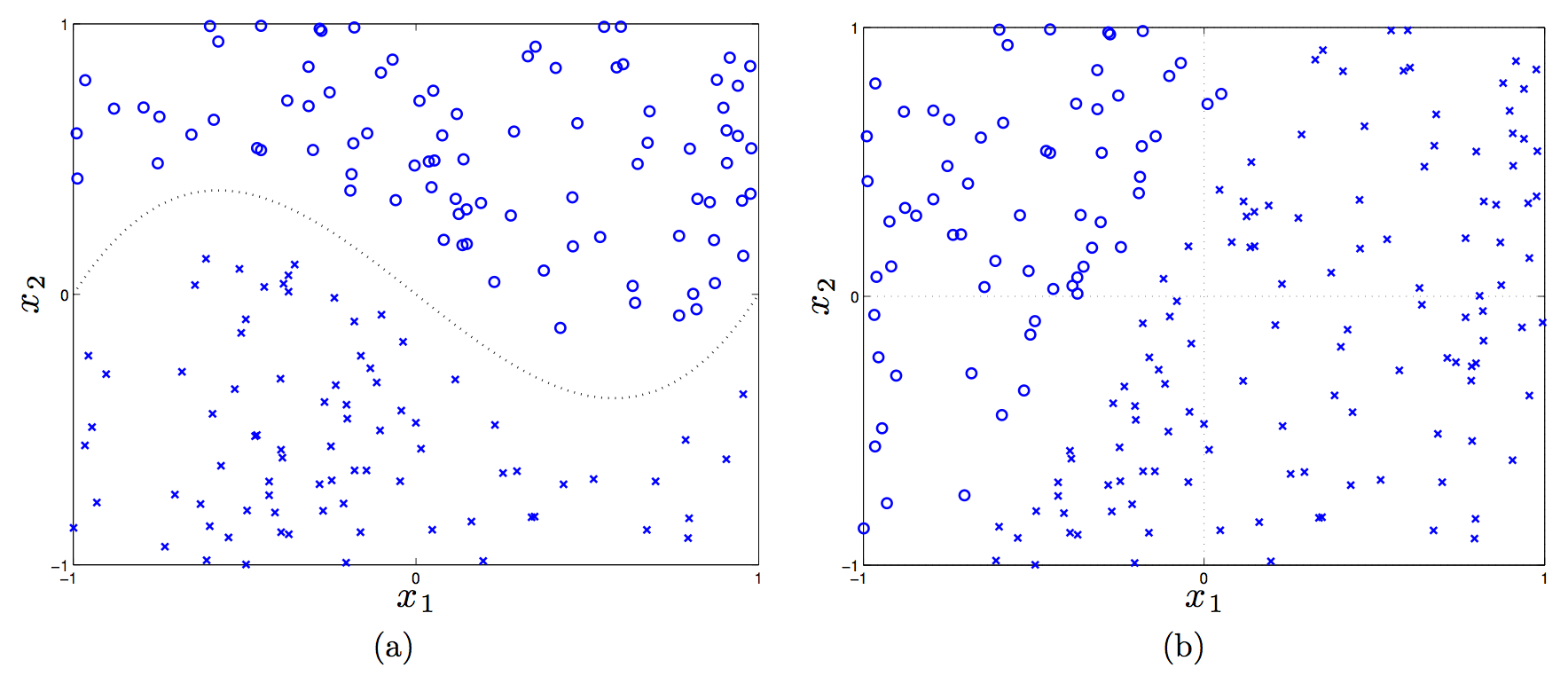
(In the first plot, the dotted line is \(f(x_1) = x_1^3 - x_1\).)

Let’s consider a linear, a shifted linear, a quadratic, and cubic kernels (see the handout for details on these), and see if any of them can linearly separate the data in the two plots.

Plot (a) requires a third-order polynomial to separate the data, so only the cubic kernel will work, because that will map feature vectors \(x \to \phi(x)\) to have \(x_1^3\) in it. Then we’d just adjust the weights to set that to have nonzero weight.

In plot (b), a linear kernel is enough, but there has to be a bias term in there! (That actually tricked me.) Without a bias, in the 2-D case here, the decision rule is \({\rm sign}(w^Tx)\), and a 2-D vector \(w\) must “emanate” out of the origin, which means the perpendicular line to it crosses the origin.

Kernels, Formalized

The preceding discussion motivates the following question: how do we know if a function \(K\) is a valid kernel? First, the official definition of a kernel is that it is a function \(K(x,y) = \phi(x)^T\phi(y)\) that performs an inner product in a Hilbert Space. Normally, I prefer thinking of the inner product \(\langle \phi(x),\phi(y) \rangle\) as the normal dot product (as I wrote earlier) but more generally, we should use the terminology of the inner product. Those satisfy properties of symmetry, bilinearity, and positive definiteness. A Hilbert Space is an inner product space that is complete and separable with respect to the norm defined by the inner product.

Since we are only dealing with real-valued vectors, our Hilbert Space will be \(\mathbb{R}^n\) and the inner product here is the normal vector dot product. To test whether a function is a kernel, we invoke a simplified form of Mercer’s Theorem: let function \(K : \mathbb{R}^n \times \mathbb{R}^n \to \mathbb{R}\) be given. Then for \(K\) to be a valid Mercer kernel, it is necessary and sufficient that for any set of points \(\{x^{(1)}, \ldots, x^{(m)}\}\) the corresponding kernel matrix is (symmetric) positive semi-definite. The element \(K_{ij}\) of the kernel matrix is the value \(K(x^{(i)},x^{(j)})\). (Sometimes the kernel matrix is called the Gram matrix.)

To prove one direction, that if \(K\) is a kernel matrix corresponding to a feature mapping \(\phi\), it must be symmetric positive semi-definite, we proceed as follows. First, it’s going to be symmetric due to the dot product (or more accurately, inner product) being commutative. Next, for any \(z \in \mathbb{R}^n\), we have

where we used the fact we indirectly showed earlier that \(\sum_i\sum_j x_iz_ix_jz_j = (x^Tz)^2 \ge 0\). It’s a little tricky because we are keeping \(k\), a component of \(\phi\), fixed, and ranging across different \(\phi\) vectors.

This fact about positive semi-definiteness makes it easy to see that the following are also valid kernels:

• Addition: \(K_1 + K_2\)
• Multiplication: \(K^T K\)
• Scalar: \(cK\) for a constant \(c \ge 0\)

We can use kernels for perceptrons (as previously discussed), support vector machines (as we will discuss), principal components analysis, and other classifiers such as linear regression.

Let’s discuss the linear regression case. In the general (regularized) case, the objective is:

where \(X\) is the \(n \times m\) matrix of training instances, where each training instance is a row (this is different from what I usually think of it, but it makes more sense in regression). The \(y \in \mathbb{R}^n\) vector has the true labels. By taking derivatives, we see that the optimal \(w\) is

In the last step above, I used the clever trick I learned from CS 281A that for \(\lambda > 0\) and a matrix \(A\) that is \(d\times n\), we have \((AA^T + \lambda I)^{-1}A = A(A^TA + \lambda I)^{-1}\). But wait, what does this mean? We can express \(w\) as

with an appropriately defined \(\alpha_i\) since the columns of \(X^T\) (not \(X\), be careful!) are the actual training elements, so \(w\) is in the space spanned by them and thus we can write it as a linear combination.

When we are faced with a new training instance to do regression, \(x_{\rm new}\), we will perform the following:

We have kernels again! This is more accurately known as kernelized linear regression. In fact, we even use kernels before we test on new examples (i.e., we use it during training). Why? The matrix \(XX^T\) is itself a kernel matrix! It consists of dot products between the training instances, and since we optimize over that during training, we will use kernels during training.

I may end up reading more of Tom Mitchell’s slides on this, because this was quite illuminating to me.

Support Vector Machines

We now switch gears to Support Vector Machines (SVMs), which are possibly the best “off-the-shelf” classifier because they combine the kernel trick along with the concept of a maximum margin separator. Thus, we know immediately that – like in the perceptron – we must find some way to express the optimization problem in terms of dot products.

To begin the derivation, we define the functional margin of a weight vector \((w,b)\) (note: we keep the intercept term separate now) with respect to training instance \(x^{(i)}\) to be \(\gamma^{(i)} = y^{(i)}(w^Tx^{(i)}+b)\), where the class label \(y^{(i)} \in \{-1,1\}\), and across the entire dataset, \(\gamma\) is just the minimum of all the functional margins. Ideally, we would like the functional margin to be relatively large, as that would indicate a strong, “robust” boundary between the two classes.

We can formulate SVMs with the following “optimization” problem:

such that

along with the restriction that \(\|w\|_2 = 1\), which prevents the functional margin from changing due to invariance of the size of \(w\) (though \(b\) might vary, but I don’t think it’s a problem).

Unfortunately, this is not really possible with “optimization” easily, so we transform the problem into an equivalent one as follows:

such that for all training instances \(i \in \{1,2,\ldots,m\}\), we have the constraint \(y^{(i)}(w^Tx^{(i)} + b) \ge 1\). This scales \(w,b\) so that the functional margin must be one.

We are done, but it is better to face the problem from the dual perspective so that we can take advantage of kernels. Since the dual solution \(d^*\) is less than or equal to the primal solution \(p^*\), it follows that we can equivalently solve the problem by maximizing the dual⁴. We re-write the constraints as \(g_i(w) = 1-y^{(i)}(w^Tx^{(i)}+b) \le 0\) and construct the Lagrangian as:

Setting the derivative of \(\mathcal{L}\) with respect to \(w\) and \(b\), then after some algebra (which took me a while due to lots of indices messing me up, but I eventually got it), and then knowing that we need to maximize this, we pose the dual optimization problem:

such that \(\alpha_i \ge 0\) for all \(i\), and \(\sum_{i=1}^m \alpha_iy^{(i)} = 0\). Fortunately, this is convex, so there is a single global minimum.

Notice that we have \(\alpha\) variables again, though these have a different interpretation than the ones in the kernelized perceptron, though. Watch out! And yes, we do get kernels to appear once again. Nice!

Now let’s see what happens when we have trained and are going to assign a class to a new instance \(x_{\rm new}\). We perform the \({\rm sign}(w^Tx_{\rm new}+b)\) computation, which can equivalently be expressed as

Once again, we have kernels! Incidentally, it looks like we might have to do a lot of computation for classifying a single point, but in fact, most of the \(\alpha_i\)s will be zero. The few that are nonzero correspond to the training instances called support vectors, and they are the ones closest to the margin. This is formally called the Karush-Kuhn-Tucker dual complementarity condition. The fact that we may not need to do much computation means SVMs gain some of the advantages of parametric models.

In the above problem, we – just like in the kernelized perceptron and kernelized regression – have formulated the problem so that, both during training and classification of new examples, the data enter via inner products, allowing us to use kernels.

What happens when we do not have linearly separable data? Rather than come up with a more complicated or longer feature vector (which might risk overfitting), we can reformulate the problem using slack variables (for \(\ell_1\)-regularization) and an additional, controllable parameter \(C\):

such that for all \(i \in \{1,2,\ldots,m\}\), we have \(y^{(i)}(w^Tx^{(i)}+b) \ge 1 - \xi_i\) and \(\xi_i \ge 0\). Thus, samples are permitted to have a (functional) margin less than one.

Rather surprisingly, the only change to the dual is that \(\alpha_i \ge 0\) constraints turns into \(C \ge \alpha_i \ge 0\) constraints, so we can apply the same principles (roughly speaking) as we did in the linearly separable case. In addition, the way we find \(b\) changes, but generally we don’t really worry about the intercept too much when going through the derivation. It’s really \(w\) that matters most to me.