This post serves as a continuation of my last post on the fundamentals of policy gradients. Here, I continue it by discussing the Generalized Advantage Estimation (arXiv link) paper from ICLR 2016, which presents and analyzes more sophisticated forms of policy gradient methods.

Recall that raw policy gradients, while unbiased, have high variance. This paper proposes ways to dramatically reduce variance, but this unfortunately comes at the cost of introducing bias, so one needs to be careful before applying tricks like this in practice.

The setting is the usual one which I presented in my last post, and we are indeed trying to maximize the sum of rewards (assume no discount). I’m happy that the paper includes a concise set of notes summarizing policy gradients:

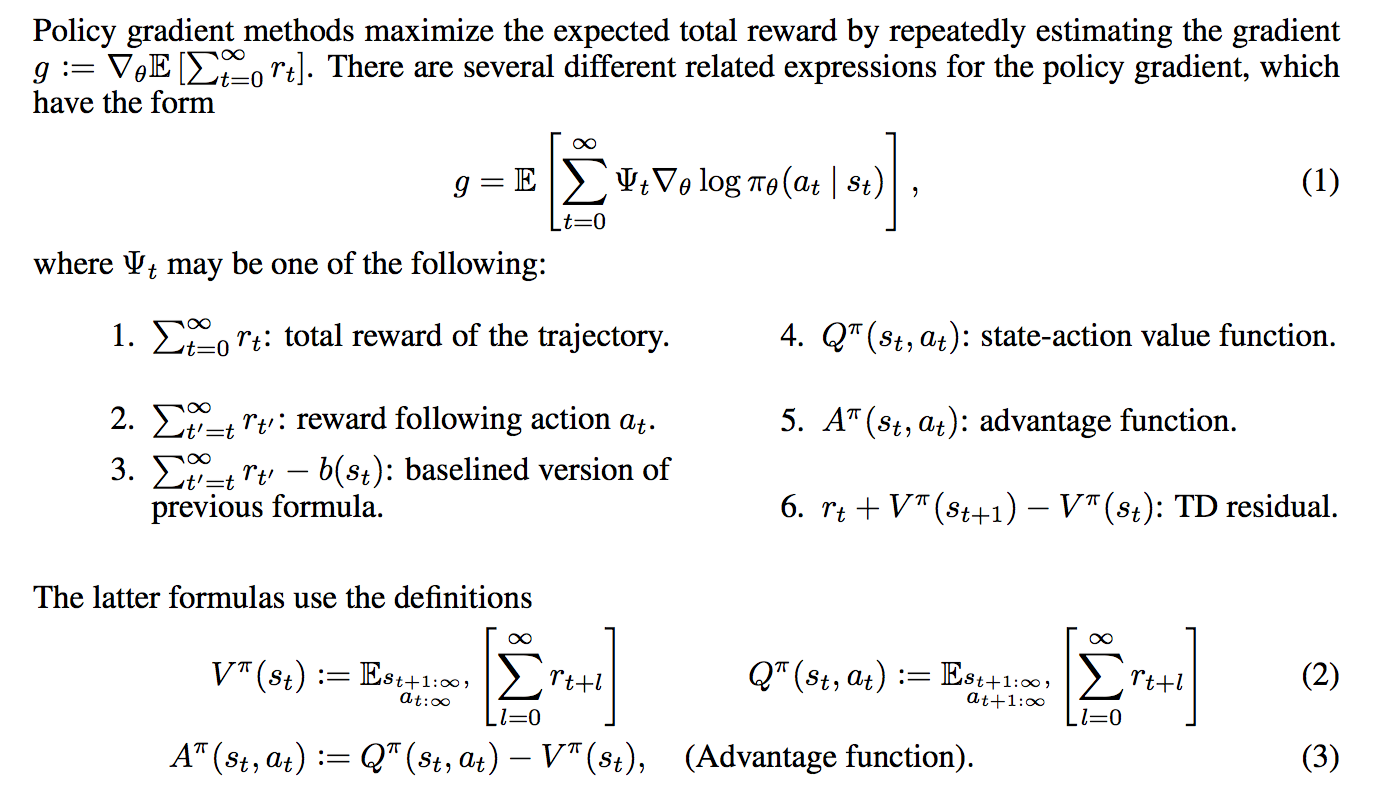
If the above is not 100% clear to you, I recommend reviewing the basics of policy gradients. I covered five of the six forms of the \(\Psi_t\) function in my last post; the exception is the temporal difference residual, but I will go over these later here.

Somewhat annoyingly, they use the infinite-horizon setting. I find it easier to think about the finite horizon case, and I will clarify if I’m assuming that.

Proposition 1: \(\gamma\)-Just Estimators.

One of the first things they prove is Proposition 1, regarding “\(\gamma\)-just” advantage estimators. (The word “just” seems like an odd choice here, but I’m not complaining.) Suppose \(\hat{A}_t(s_{0:\infty},a_{0:\infty})\) is an estimate of the advantage function. A \(\gamma\)-just estimator (of the advantage function) results in

This is for one time step \(t\). If we sum over all time steps, by linearity of expectation we get

In other words, we get an unbiased estimate of the discounted gradient. Note, however, that this discounted gradient is different from the gradient of the actual function we’re trying to optimize, since that was for the undiscounted rewards. The authors emphasize this in a footnote, saying that they’ve already introduced bias by even assuming the use of a discount factor. (I’m somewhat pleased at myself for catching this in advance.)

The proof for Proposition 1 is based on proving it for one time step \(t\), which is all that is needed. The resulting term with \(\hat{A}_t\) in it splits into two terms due to linearity of expectation, one with the \(Q_t\) function and another with the baseline. The second term is zero due to the baseline causing the expectation to zero, which I derived in my previous post in the finite-horizon case. (I’m not totally sure how to do this in the infinite horizon case, due to technicalities involving infinity.)

The first term is unfortunately a little more complicated. Let me use the finite horizon \(T\) for simplicity so that I can easily write out the definition. They argue in the proof that:

Most of this proceeds by definitions of expectations and then “pushing” integrals into their appropriate locations. Unfortunately, I am unable to figure out how they did step (i). Specifically, I don’t see how the integral over \(a_t\) somehow “moves past” the \(\nabla_\theta \log \pi_\theta(a_t|s_t)\) term. Perhaps there is some trickery with the law of iterated expectation due to conditionals? If anyone else knows why and is willing to explain with detailed math somewhere, I would really appreciate it.

For now, I will assume this proposition to be true. It is useful because if we are given the form of estimator \(\hat{A}_t\) of the advantage, we can immediately tell if it is an unbiased advantage estimator.

Advantage Function Estimators

Now assume we have some function \(V\) which attempts to approximate the true value function \(V^\pi\) (or \(V^{\pi,\gamma}\) in the undiscounted setting).

• Note I: \(V\) is not the true value function. It is only our estimate of it, so \(V_\phi(s_t) \approx V^\pi(s_t)\). I added in the \(\phi\) subscript to indicate that we use a function, such as a neural network, to approximate the value. The weights of the neural network are entirely specified by \(\phi\).

• Note II: we also have our policy \(\pi_\theta\) parameterized by parameters \(\theta\), again typically a neural network. For now, assume that \(\phi\) and \(\theta\) are separate parameters; the authors mention some enticing future work where one can share parameters and jointly optimize. The combination of \(\pi_{\theta}\) and \(V_{\phi}\) with a policy estimator and a value function estimator is known as the actor-critic model with the policy as the actor and the value function as the critic. (I don’t know why it’s called a “critic” because the value function acts more like an “assistant”.)

Using \(V\), we can derive a class of advantage function estimators as follows:

These take on the form of temporal difference estimators where we first estimate the sum of discounted rewards and then we subtract the value function estimate of it. If \(V = V^{\pi,\gamma}\), meaning that \(V\) is exact, then all of the above are unbiased estimates for the advantage function. In practice, this will not be the case, since we are not given the value function.

The tradeoff here is that the estimators \(\hat{A}_t^{(k)}\) with small \(k\) have low variance but high bias, whereas those with large \(k\) have low bias but high variance. Why? I think of it based on the number of terms. With small \(k\), we have fewer terms to sum over (which means low variance). However, the bias is relatively large because it does not make use of extra “exact” information with \(r_K\) for \(K > k\). Here’s another way to think of it as emphasized in the paper: \(V(s_t)\) is constant among the estimator class, so it does not affect the relative bias or variance among the estimators: differences arise entirely due to the \(k\)-step returns.

One might wonder, as I originally did, how to make use of the \(k\)-step returns in practice. In Q-learning, we have to update the parameters (or the \(Q(s,a)\) “table”) after each current reward, right? The key is to let the agent run for \(k\) steps, and then update the parameters based on the returns. The reason why we update parameters “immediately” in ordinary Q-learning is simply due to the definition of Q-learning. With longer returns, we have to keep the Q-values fixed until the agent has explored more. This is also emphasized in the A3C paper from DeepMind, where they talk about \(n\)-step Q-learning.

The Generalized Advantage Estimator

It might not be so clear which of these estimators above is the most useful. How can we compute the bias and variance?

It turns out that it’s better to use all of the estimators, in a clever way. First, define the temporal difference residual \(\delta_t^V = r_t + \gamma V(s_{t+1}) - V(s_t)\). Now, here’s how the Generalized Advantage Estimator \(\hat{A}_t^{GAE(\gamma,\lambda)}\) is defined:

To derive this, one simply expands the definitions and uses the geometric series formula. The result is interesting to interpret: the exponentially-decayed sum of residual terms.

The above describes the estimator \(GAE(\gamma, \lambda)\) for \(\lambda \in [0,1]\) where adjusting \(\lambda\) adjusts the bias-variance tradeoff. We usually have \({\rm Var}(GAE(\gamma, 1)) > {\rm Var}(GAE(\gamma, 0))\) due to the number of terms in the summation (more terms usually means higher variance), but the bias relationship is reversed. The other parameter, \(\gamma\), also adjusts the bias-variance tradeoff … but for the GAE analysis it seems like the \(\lambda\) part is more important. Admittedly, it’s a bit confusing why we need to have both \(\gamma\) and \(\lambda\) (after all, we can absorb them into one constant, right?) but as you can see, the constants serve different roles in the GAE formula.

To make a long story short, we can put the GAE in the policy gradient estimate and we’ve got our biased estimate (unless \(\lambda=1\)) of the discounted gradient, which again, is itself biased due to the discount. Will this work well in practice? Stay tuned …

Reward Shaping Interpretation

Reward shaping originated from a 1999 ICML paper, and refers to the technique of transforming the original reward function \(r\) into a new one \(\tilde{r}\) via the following transformation with \(\Phi: \mathcal{S} \to \mathbb{R}\) an arbitrary real-valued function on the state space:

Amazingly, it was shown that despite how \(\Phi\) is arbitrary, the reward shaping transformation results in the same optimal policy and optimal policy gradient, at least when the objective is to maximize discounted rewards \(\sum_{t=0}^\infty \gamma^t r(s_t,a_t,s_{t+1})\). I am not sure whether the same is true with the undiscounted case as they have here, but it seems like it should since we can set \(\gamma=1\).

The more important benefit for their purposes, it seems, is that this reward shaping leaves the advantage function invariant for any policy. The word “invariant” here means that if we computed the advantage function \(A^{\pi,\gamma}\) for a policy and a discount factor in some MDP, the transformed MDP would have some advantage function \(\tilde{A}^{\pi,\gamma}\), but we would have \(A^{\pi,\gamma} = \tilde{A}^{\pi,\gamma}\) (nice!). This follows because if we consider the discounted sum of rewards starting at state \(s_t\) in the transformed MDP, we get

“Hitting” the above values with expectations (as Michael I. Jordan would say it) and substituting appropriate values results in the desired \(\tilde{A}^{\pi,\gamma}(s_t,a_t) = A^{\pi,\gamma}(s_t,a_t)\) equality.

The connection between reward shaping and the GAE is the following: suppose we are trying to find a good policy gradient estimate for the transformed MDP. If we try to maximize the sum of \((\gamma \lambda)\)-discounted sum of (transformed) rewards and set \(\Phi = V\), we get precisely the GAE! With \(V\) here, we have \(\tilde{r}(s_t,a_t,s_{t+1}) = \delta_t^V\), the residual term defined earlier.

To analyze the tradeoffs with \(\gamma\) and \(\lambda\), they use a response function:

Why is this important? They state it clearly:

The response function lets us quantify the temporal credit assignment problem: long range dependencies between actions and rewards correspond to nonzero values of the response function for \(l \gg 0\).

These “long-range dependencies” are the most challenging part of the credit assignment problem. Then here’s the kicker: they argue that if \(\Phi = V^{\pi,\gamma}\), then the transformed rewards are such that \(\mathbb{E}[\tilde{r}_{l+t} \mid s_t,a_t] - \mathbb{E}[\tilde{r}_{l+t} \mid s_t] = 0\) for \(l>0\). Thus, long-range rewards have to induce an immediate response! I’m admittedly not totally sure if I understand this, and it seems odd that we only want the response function to be nonzero at the current time (I mean, some rewards have to be merely a few steps in the future, right?). I will take another look at this section if I have time.

Value Function Estimation

In order to be able to use the GAE in our policy gradient algorithm (again, this means computing gradients and shifting the weights of the policy to maximize an objective), we need some value function \(V_\phi\) parameterized by a neural network. This is part of the actor-critic framework, where the “critic” provides the value function estimate.

Let \(\hat{V}_t = \sum_{l=0}^\infty \gamma^l r_{t+l}\) be the discounted sum of rewards. The authors propose the following optimization procedure to find the best weights \(\phi\):

where each iteration, \(\phi_{\rm old}\) is the parameter vector before the update, and

This is a constrained optimization problem to find the best weights for the value function. The constraint reminds me of Trust Region Policy Optimization, because it limits the amount that \(\phi\) can change from one update to another. The advantages with a “trust region” method are that the weights don’t change too much and that they don’t overfit to the current batch. (Updates are done in batch mode, which is standard nowadays.)

• Note I: unfortunately, the authors don’t use this optimization procedure exactly. They use a conjugate gradient method to approximate it. But think of the optimization procedure here since it’s easier to understand and is “ideal.”

• Note II: remember that this is not the update to the policy \(\pi_\theta\). That update requires an entirely separate optimization procedure. Don’t get confused between the two. Both the policy and the value functions can be implemented as neural networks, and in fact, that’s what the authors do. They actually have the same architecture, with the exception of the output layer since the value only needs a scalar, whereas the policy needs a higher-dimensional output vector.

Putting it All Together

It’s nice to understand each of the components above, but how do we combine them into an actual algorithm? Here’s a rough description of their proposed actor-critic algorithm, each iteration:

• Simulate the current policy to collect data.

• Compute the Bellman residuals \(\delta_{t}^V\).

• Compute the advantage function estimate \(\hat{A}_t\).

• Update the policy’s weights, \(\theta_{i+1}\), with a TRPO update.

• Update the critic’s weights, \(\phi_{i+1}\), with a trust-region update.

As usual, here are a few of my overly-detailed comments (sorry again):

• Note I: Yes, there are trust region methods for both the value function update and the policy function update. This is one of their contributions. (To be clear, the notion of a “GAE” isn’t entirely their contribution.) The value and policy are also both neural networks with the same architecture except for the output since they have different outputs. Honestly, it seems like we should always be thinking about trust region methods whenever we have some optimization to do.

• Note II: If you’re confused by the role of the two networks, repeat this to yourself: the policy network is for determining actions, and the value network is for improving the performance of the gradient update (which is used to improve the actual policy by pointing the gradient in the correct direction!).

They present some impressive experimental benchmarks using this actor-critic algorithm. I don’t have too much experience with MuJoCo so I can’t intuitively think about the results that much. (I’m also surprised that MuJoCo isn’t free and requires payment; it must be by far the best physics simulator for reinforcement learning, otherwise people wouldn’t be using it.)

Concluding Thoughts

I didn’t understand the implications of this paper when I read it for the first time (maybe more than a year ago!) but it’s becoming clearer now. They present and analyze a specific kind of estimator, the GAE, which has a bias-variance “knob” with the \(\lambda\) (and \(\gamma\), technically). By adjusting the knob, it might be possible to get low variance, low biased estimates, which would drastically improve the sample efficiency of policy gradient methods. They also present a way to estimate the value method using a trust region method. With these components, they are able to achieve high performance on challenging reinforcement learning tasks with continuous control.