Notes on Exact Inference in Graphical Models

In an effort to help me understand certain topics better for my prelim exam next month, I thought I’d briefly write about a topic that I sometimes never feel like I understand completely: exact inference in graphical models. Given a graphical model, inference is simply the task of computing the probability $P(X = x \mid E = e)$, where \(X\) is a set of query variables, \(E\) is a set of evidence variables, and if we include another disjoint set \(H\) of the hidden variables, then \(X \cup E \cup H\) represents the entire set of nodes in the graphical model. In general, inference is intractable, but for now we’ll pretend not to worry about that by discussing two ways of doing exact inference: by enumeration, and by variable elimination.

Inference by Enumeration

Here’s an example of a Bayesian Network, i.e., a directed graphical model with seven variables. This comes from the spring 2011 final for Berkeley’s undergraduate AI course, and the reason why there’s one \(Y\) but six \(X_i\)s is because the question using this graphical model wanted to emphasize how the \(Y\) represented a class variable. But it’s still a variable, just like all the $X_i$s, so the distinction is not important now.

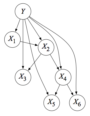
Suppose we want to compute the exact quantity of¹ \(P(X_2 = x_2 \mid X_4 = x_2)\). The first key point we need to know is that this computation immediately reduces to the computation of the joint \(P(X_2 = x_2, X_4 = x_4)\), which directly follows from the definition of the conditional probability. Once we compute that joint, we can then divide by \(P(X_4 = x_4)\). Or, better yet, since the denominator does not depend on the value we choose for \(X_2\), we can avoid computing it by determining \(P(X_2, X_4=x_4)\) while substituting in the possible states of \(x_2\). These values will give us the normalizing constant we need, because we will be computing a vector of probabilities (one element per assignment to \(X_2\)) and the normalizing constant is the sum of all those elements. The point of all this previous discussion is this: the computation of conditional probabilities immediately reduces to the computation of joint probabilities.

Joint probabilities are easier for me to digest. In the current example, the joint can be re-expressed (using the simpler form of omitting the capital variables) as

Notice that we split up the joint into the conditionals described by the network, and then pushed the summations as far right as possible. The notation \(\sum_y P(y)\) means that if \(Y \in \{1,2,3\}\), we are determining \(P(Y=1)+P(Y=2)+P(Y=3)\), i.e., we sum over the possible states of \(Y\). So, in the above algebra, we sum over the possible set of states for the variables other than \(X_2\) and \(X_4\), which are assumed fixed, but we still denote their values \(x_2\) and \(x_4\) with lowercase variables. Sorry. As my former professor Ben Recht would say, “the worst part about this is the notation.”

We need to be careful to make sure that we are rearranging the sums and probabilities correctly. For instance, \(P(y)\) is all the way to the left because it only depends on \(Y\), but so is \(P(x_4\mid x_2,y)\)! The reason is, again, that \(X_4\) and \(X_2\) are fixed to those values, so there is no dependency over any other summation.

At this point, exact inference by enumeration simply means computing the quantity above from left to right. So we would first fix \(Y\) to a state, then compute \(P(y)P(x_4\mid x_2,y)\), then loop over the values for \(X_1\), and so on. It’s basically like how we have nested for loops in computer programming. This will give us the exact values. Then we have our desired conditional determined up to proportion: \(P(x_2\mid x_4) \propto P(x_2,x_4)\). To get the exact value, repeat the computation for all states of \(X_2\).

Variable Elimination

Variable elimination is the same as inference by enumeration, except for two things: (1) that we compute right to left and that (2) the exact order of our summations will change based on our variable ordering. That’s it! The key advantage of variable elimination over enumeration is that variable elimination is a dynamic programming algorithm and re-uses computation.

I’m not going to go through the entire variable elimination algebra here, because the notation is tedious and we will do an example later, but here would be the first step. In the math above, we would transform \(\sum_{x_6} P(x_6\mid x_4,y)\) into an intermediate factor \(m_6(y)\), where the subscript 6 denotes the variable we just eliminated, and \(y\) indicates the variable it depends on (it does not depend on the “variable” \(x_4\) because it is fixed, but we are still summing over values of \(Y\))². Then we repeat the process by creating more intermediate factors by going right to left. If we had to re-do a lot of computations in enumeration, then variable elimination will save us lots of computation time.

Some notes:

• It is possible to view variable elimination in a graph-theoretic way on undirected graphs. Here’s what happens: for a Markov Random Field, we use the graph directly, and for a Bayesian Network (like the one above), we would first moralize the graph by iterating through each node in the graph, connecting its parents, and then dropping the orientation of its edges. Great, so now we have an undirected graph – what now? First, we need a variable elimination ordering where the query variable (\(X_2\) in the above example) is listed last³. Then, for each variable in the ordering, we eliminate it. For a variable \(Z\), this means – graphically – that we would connect all neighbors of \(Z\) with an undirected edge (this forms a clique!), then eliminate \(Z\) from the graph. We repeat this process for all variables, until we get to our query variable, upon which time we will know the value of interest for the probability.

• The order in which we eliminate variables is crucially important. This is beyond the scope of this post, but the run time of variable elimination is dominated by the size of the largest clique formed in the graph-theoretic version I just described. This is formalized as the treewidth of the graph, which is defined as one less than the size of the largest clique formed, in the best possible variable ordering for the graph. Unfortunately, it is intractable to know the optimal variable ordering, but we can have heuristics.

I need to add a word of caution to the first bullet point above. There are different ways of interpreting variable elimination⁴. Some sources do not include the query variables in the elimination ordering, because it is assumed fixed (and it is always last so why bother). Similarly, some would also not include the evidence variables (\(x_4\) in our case) because we are not “eliminating” them. To me, it is a little unclear how this works graphically. What happens when we eliminate a variable that is connected to an evidence or query variable? Do we have to add edges between pairs of nodes where at least one is a query or evidence node? Do we eventually delete the evidence nodes? (We would never delete the query one because it is always last and by the time we finish, that node is the only thing left in the graph.) For now, my interpretation is that I’ll keep the query and evidence variables in the graph⁵. If we eliminate a neighbor, we just don’t add edges to those nodes, because there is no “interaction” with those variables – again, the query and evidence values are fixed. If we end up with no edges towards one of the evidence variables at any point in the query, then I guess we can finally remove the node. My definition of elimination means that we can only “eliminate” a variable that corresponds to one of the summations \(\sum_x\) in the above algebra.

Variable elimination – like inference by enumeration – takes exponential time in the worst case, based on the size of the conditional probability tables of the graphical model. In practice, as long as a graph of interest has a small enough treewidth (which usually means up to three), we can apply the algorithm. In a special class of graphs known as polytrees, inference takes (gasp) linear time!

With that said, we now turn to an example to apply our knowledge.

Example

Now let’s get back to that original question on the spring 2011 Berkeley AI final exam. I find practice exams (with solutions) to be among the gold mine for learning. Sometimes I learn more from practice finals than by reading an entire textbook! So it’s worth the time to go over the questions. The solutions key is already online, but for the variable elimination questions, I will go over the algebra and discuss the answers in more depth.

Here’s part (a):

Suppose we observe no variables as evidence in the TANB above. What is the classification rule for the TANB? Write the formula in terms of the CPTs (Conditional Probability Tables) and prior probabilities in the TANB

This isn’t really graphical-model related, because it’s simply \(\arg \max_y P(y)\). We could re-express \(P(y)\) with the other six variables if we have the patience to write out six \(\sum_x\)s.

Here’s part (b):

Assume we observe all the variables \(X_1 = x_1,X_2 = x_2,\ldots,X_6 = x_6\) in the TANB above. What is the classification rule for the TANB? Write the formula in terms of the CPTs and prior probabilities in the TANB.

Now we really do have to write things out explicitly, because the classification rule is \(\arg \max_y P(y,x_1,x_2,x_3,x_4,x_5,x_6)\), with all variables fixed (except for \(Y\), but we are fixing it here when we have to try different values of \(y\)). Here’s the joint I wrote earlier but will repeat here:

\(P(y)P(x_1\mid y)P(x_2\mid x_1,y)P(x_3\mid x_2,y)P(x_4\mid x_2,y)P(x_5\mid x_4,y)P(x_6\mid x_4,y)\).

We will have to use this joint in part (c), which finally introduces us to variable elimination:

Specify an elimination order that is efficient for the query \(P(Y \mid X_5 = x_5)\) in the TANB above (the query variable \(Y\) should not be included your ordering). How many variables are in the biggest factor (there may be more than one; if so, list only one of the largest) induced by variable elimination with your ordering? Which variables are they?

Now things get interesting. How do we determine an efficient variable elimination? The idea is that we come up with an ordering, then see the \(m_i(x_j,\ldots)\)s we get, and make sure that the largest \(m_i\) function is “not too large.”

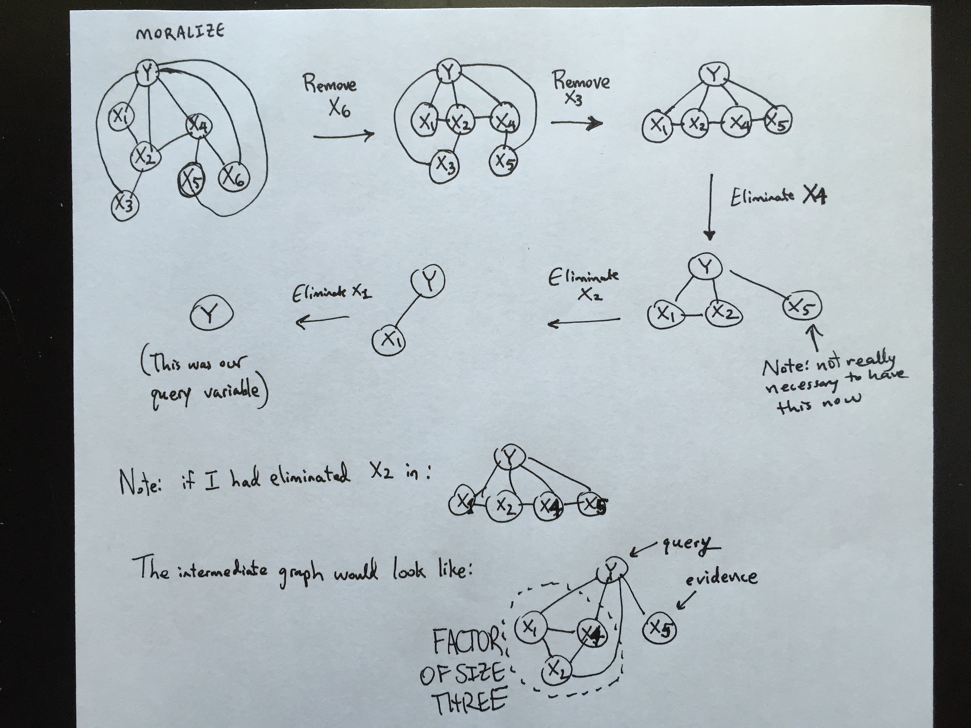
A useful first step that I use is that, after moralizing the graph, I see if there is any variable I can eliminate that will not create any additional edges. First, I notice that the variables \(X_3\) and \(X_6\) both have the property that their parents are connected in the moralized graph. Thus, removing those two variables should not add new edges, and so the largest clique will remain small. The clique will be of size two, as we are not counting the evidence or query variables.

It then remains to determine an ordering for \(\{X_1,X_2,X_4\}\). For that, I would look at the moralized graph with edges removed or added (none added in this case so far), and then try and see if I could eliminate nodes that would involve creating as few new edges as possible. The following picture shows my drawing of the variable elimination, because it would have taken forever to typeset this in LaTeX using the tikz library. Spoiler alert: I’ve already done the full elimination. I will describe why it makes sense to do this shortly.

Algebraically, this corresponds to the following⁶, a right-to-left evaluation where we start with the full joint and then shift the summations and probabilities around:

Notice that indeed, it makes sense to get rid of \(X_3\) and \(X_6\) since they are simple cases that sum away to one. In fact, the solutions manual says that these variables should not even be included in a variable elimination ordering.

Next, we have to consider some combination of \(X_1,X_2,\) and \(X_4\) to eliminate. The ordering here does matter! Here’s why: both \(X_1\) and \(X_4\) are connected to one other variable (\(X_2\)) and the two other nodes that represent fixed values. But \(X_2\) is connected to two other variables! So if we tried to eliminate \(X_2\) first, we would create an edge between \(X_1\) and \(X_4\) before removing \(X_2\) from the graph, creating a factor of size three. Algebraically, this is:

Notice what happened! The \(m_2(x_1,x_4)\) function has two arguments, which is one more than anything we did in the optimal ordering above, which was \(\{X_4,X_2,X_1\}\).

Thus, the elimination ordering must have one of \(X_1\) or \(X_4\). Then, we can do \(X_2\). In fact, after we pick the first of \(X_1\) or \(X_4\), it doesn’t matter what order the last two are eliminated. Remember that we are not including \(Y\) here because it should technically be a fixed variable: we want to pick different values \(Y=y\) to run variable elimination.

The size of the largest factor here should be two, again, assuming that we do not count the fixed variables of \(Y\) or \(X_5\) in these cliques.

Whew! Hopefully all the above analysis is clear.

To my delight, variable elimination continues in part (d):

Specify an elimination order that is efficient for the query \(P(X_3 \mid X_5 = x_5)\) in the TANB above (including \(X_3\) in your ordering). How many variables are in the biggest factor (there may be more than one; if so, list only one of the largest) induced by variable elimination with your ordering? Which variables are they?

Unfortunately, the situation is not as easy as it was last time, because now we are forced to generate an \(m_i(...)\) function that will have two arguments, so the largest factor size is three. Also, note that now we want \(X_3\) in the ordering. I’m not sure why this is the case since \(Y\) was not included in the last part, but it doesn’t make much of a difference because we know query variables should always be last, so \(X_3\) will be last in the ordering. Now we will determine the other five variables (this excludes \(X_5\) because it is fixed).

As usual, first we check if there is a way we can arrange the sums so that a variable can be summed out as one. Looking at the moralized graph, we can still remove \(X_6\) as we did last time, for the same reasons. Thus, our probabilities would start out as:

Unfortunately, looking at the resulting (moralized) graph without \(X_6\) (it’s the same as the first graph listed in my image above), there is just no way to eliminate one of \(\{Y,X_1,X_2,X_4\}\) without adding an edge. We can no longer treat \(Y\) as a fixed variable.

Here’s one possible ordering: \(X_4,X_1,X_2,Y,X_3\). The algebra is as follows:

Notice that the largest factor size will be three, which here was created twice, once with \(\{X_4,X_2,Y\}\), and the other with \(\{X_1,X_2,Y\}\). Notice that if we had tried eliminating \(Y\) (or \(X_2\)) right after \(X_6\), then we would have created a size four factor/clique involving \(\{Y,X_1,X_2,X_4\}\)! Again, all of these factor computations assume that fixed variables (query or evidence) do not count.

We gain a little more insight about variable elimination with part (e):

Does it make sense to run Gibbs sampling to do inference in a TANB? In two or fewer sentences, justify your answer.

Gibbs sampling is an approximate inference algorithm, which we use if exact inference is intractable. But here? Come on, we only have seven variables, and the treewidth of this graph is small; even for the query in part (d), our largest factor was of size three, so the clique would be size two. There is no reason to be approximate here.

The remaining parts do not have much of an emphasis on variable elimination, so I’ll just refer you to the exam and solutions key if you want to take a look.

Anyway, those are my thoughts on exact inference in graphical models, with an emphasis on enumeration and (especially) variable elimination.