Expectation-Maximization

All right, I lied in the title of my last post. That wasn’t the final word on graphical models after all¹. In this post, we’ll discuss Expectation-Maximization, which is an incredibly useful and widespread algorithm in machine learning, though many in the field view it as “hacking” due to its lack of statistical guarantees². At first, I wasn’t sure what this had to do with graphical models. True, it’s not what I’d call core graphical models, but what happens is that a lot of problems that “factor” into nice Bayesian Network representations can use Expectation Maximization to determine the optimal value of their parameters (which are CPTs in the Bayesian Network case).

The Formalities of Expectation-Maximization

Expectation-Maximization (EM) is an extremely useful algorithm that applies in cases when we have a model with unobserved (i.e., latent) variables, and we need to train the model parameters despite the lack of that information. Why do we want latent variables? It helps to simplify our models. The canonical example is seeing a bunch of health measurements, then adding in a hidden node that represents the presence of heart disease.

We apply EM when we have some probabilistic model \(p(X,Z\mid \theta)\) in which we are trying to find the “best” model parameters \(\theta\), which usually means taking the Maximum Likelihood Estimate (MLE). Crucially, \(X\) is our observed variable (or a set of them), while \(Z\) represents the latent variables. Usually, we use logs when maximizing likelihood, so this is equivalent to finding \(\arg \max_\theta \log \sum_Z p(X,Z\mid \theta)\), which Mike calls the incomplete log likelihood³. This is hard; marginalization here (because it involves summing over \(Z\)) tends to “make problems harder.” My intuition: having sums means we don’t usually have a closed-form expression of the likelihood function, so how can we find the MLE for \(\theta\)?

We can define the expected complete log likelihood with some other distribution \(q(Z\mid X)\) as \(\sum_Z q(Z\mid X)\log p(X,Z\mid \theta)\), in other words, averaging out \(Z\). A good choice of \(q\) means that the expected log likelihood can be treated as the actual log likelihood.

EM is divided into two steps that repeat. Informally, the Expectation step assigns values to the hidden variables based on \(P(Z \mid X, \theta)\). (In most examples, these are indicator variables.) In the Maximization step, we find the MLE of \(\theta\), which is easy this time because we actually “know” what the \(Z\) variables are — we assigned them in the previous step!

There are two “formal perspectives” of EM, one relating to log likelihood, and the other relating to a concept known as the Kullback-Leibler Divergence.

The Log Likelihood View

Let us define the following quantity:

We further know from some algebra that \(\mathcal{L}(q,\theta) \le \log \sum_Z p(X,Z\mid \theta)\), i.e., that \(\mathcal{L}\) defines a lower bound of the incomplete log likelihood, for an arbitrary \(q\) function.

We can now define our E and M steps more precisely:

• E step: \(q^{(t+1)} = \arg \max_q \mathcal{L}(p,\theta^{(t)})\)
• M step: \(\theta^{(t+1)} = \arg \max_\theta \mathcal{L}(p^{(t+1)},\theta)\)

What does this really mean? Note that in both cases we are trying to maximize a lower bound on the incomplete log likelihood, which makes intuitive sense: that is the point of MLE!

• In the E step, we are finding the best \(q\), and this can actually be solved analytically. It’s right under our noses: \(q^{(t+1)}(Z\mid X) = p(Z\mid X,\theta^{(t)})\). I mean, that’s just the true distribution of the hidden variable, given the known data and the current parameters! It sounds obvious.

  There are two ways to show this. One is to plug in that choice of \(q\) in the function \(\mathcal{L}(p,\theta^{(t)})\), and we get equality with the incomplete log likelihood, \(\log p(X\mid \theta)\). Hence, that’s the best \(q\) we can get! The other is to take the KL-Divergence view (spoiler for the next section!) and see that

  \[\log p(X\mid \theta) - \mathcal{L}(q,\theta) = KL(q(Z\mid X)\: \| \: p(Z\mid X,\theta))\]

  which shows that to minimize the difference between the two distributions, we need to set the two distributions to be the same. Remember again that \(\mathcal{L}\) is a lower bound. I know I say this a lot, but it’s important.

• In the M step, we maximize the expected complete log likelihood, which we recall we defined earlier as \(\sum_Z q(Z\mid X)\log p(X,Z\mid \theta)\). This happens because \(\mathcal{L}(p,\theta)\) breaks into two terms, one which is the expected complete log likelihood, and the other which does not depend on \(\theta\).

Taken together, what do these steps really do? Let’s look back at the incomplete log likelihood \(\log p(X\mid \theta)\). This is hard to optimize, as we said earlier, but what the E and M steps do is that, during each iteration, they collectively keep maximizing this function! It’s a “hill climbing” algorithm that will keep increasing (or technically, never decrease) the incomplete log likelihood. Why is that the case? Here’s the intuition. The M step means that we are maximizing \(\mathcal{L}(q,\theta)\), a lower bound to the incomplete log likelihood. Hypothetically, suppose \(\mathcal{L}(q,\theta)\) was actually equal to that incomplete log likelihood. Then the M step would necessarily result in a (highly desirable!) increase in \(\log p(X\mid \theta)\). But this only works if there is equality … if there is a gap, the plan is thrown out the window.

Fortunately, the E step comes to rescue us, because we already know that for an appropriate choice of \(p\), we can get \(\mathcal{L}(p,\theta)\) to be equal to \(\log p(X\mid \theta)\). Note that the thetas here should really have a time superscript attached to them (as well as the \(p\)s) but I left them out for simplicity.

In conclusion, EM will keep increasing \(\log p(X\mid \theta)\) each iteration. This, if you recall, was the whole point of this process anyway! And it does this by cleverly optimizing the \(\mathcal{L}(q,\theta)\) function, which is much easier to handle than the incomplete log likelihood. Absolutely brilliant!

The Kullback-Leibler Divergence View

We can alternatively bound the KL-Divergence. Derive the bound

In words: the KL-divergence between the empirical distribution \(\tilde{p}(X)\) and the model \(p(X\mid \theta)\) is upper bounded by a “complete” KL-divergence. The intuition is that we are adding in the \(q(Z\mid X)\) to “average over” the values of \(Z\), just as we did earlier with the expected complete log likelihood term.

Our results carry over from the previous section because minimizing the right hand side of that expression above (with respect to \(q\) and \(\theta\)) is equivalent to maximizing \(\mathcal{L}(p,\theta)\) with respect to the same variables. Why? As part of the derivation for that bound above, we invoked \(\log p(X\mid \theta) \ge \mathcal{L}(p,\theta)\), but that part was embedded inside an expression such that there was a negation attached, so maximizing \(\mathcal{L}\) means minimizing the overall problem.

Letting \(KL(q\: \|\: \theta) = KL(\tilde{p}(X)q(Z\mid X)\: \| \: p(X,Z\mid \theta))\), the steps are:

• E step: \(q^{(t+1)} = \arg \min_q KL(q\: \| \: \theta^{(t)})\)

• M step: \(\theta^{(t+1)} = \arg \min_\theta KL(q^{(t+1)}\: \| \: \theta)\)

Example on Gaussians

This example is from Russell and Norvig (2010). It is about clustering on a dataset presumed to be generated by three unknown multivariate Gaussian distributions. Here’s an example of a plot that could represent such data, with each data point highlighted by the color of its distribution (which we would not know — they are only there for ease of readability). Note: the figure here isn’t the exact one in the textbook, but it’s close.

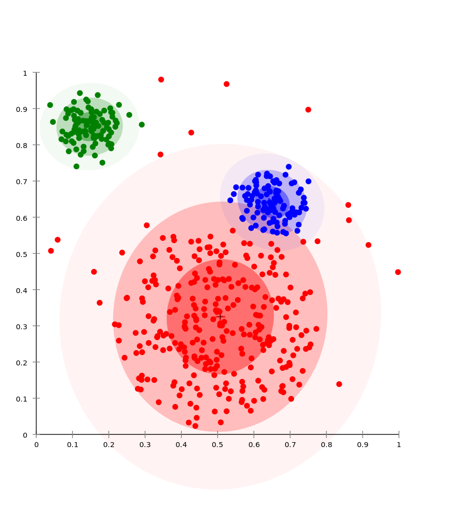
I like this example because it makes it clear how to view the \(Z\)s as indicator variables.

To formalize the problem, we assume that each data point is generated by picking one of the three two-dimensional, multivariate Gaussian distributions, then sampling from that distribution. Thus, the goal in using EM is to find the parameters of the model:

• the weight \(w_i = P(C = i)\) of each component (i.e., each multivariate Gaussian)
• the 2-dimensional mean vector \(\mu_i\) of each component
• the \(2\times 2\) covariance matrix \(\Sigma_i\) of each component

To start off with EM, we first initialize the three sets of parameters above to some random values⁴. Then we iterate:

• E step: this will determine the expected value of the hidden indicator variables in this model, which we define as \(Z_{ij}\), which is one if point \(x_j\) was generated by Gaussian component \(i\) and zero otherwise. From the earlier discussion, we know that we need to use the \(p(Z\mid X,\theta)\) function. Assuming that the points are IID, this means for each point \(x_j\), we compute \(\mathbb{E}[Z_{ij}] = p(Z_{ij}=1 \mid x_j,\theta^{(t)})\) where \(i \in \{1,2,3\}\).

  We can transform this into an easier problem using Bayes’ rule, and claim that \(p(Z_{ij} = 1 \mid x_j,\theta^{(t)}) \propto p(x_j \mid Z_{ij}=1,\theta^{(t)})p(Z_{ij} = 1\mid \theta^{(t)})\). The first quantity, \(p(x_j \mid Z_{ij}=1,\theta^{(t)})\), is a straightforward plug and chug into the formula for the density of a multivariate Gaussian, because we assume it came from the \(i\)th one, and we have the parameters \(\mu_i\) and \(\Sigma_i\) from \(\theta^{(t)}\). The second quantity, \(p(Z_{ij}=1 \mid \theta^{(t)})\) is like computing the probability that a component generated a given point, but without any dependency on any point \(j\), we just probabilistically choose based on the component’s overall weight \(w_i\), which we get from \(\theta^{(t)}\).

• M step: given the fact that we “know” which component \(i\) generated which data point \(x_j\) in a probabilistic sense, then we can find better values of the parameters using the following update equations:

  • The weights: \(w_i \leftarrow n_i/N\)
  • The means: \(\mu_i \leftarrow \sum_j \mathbb{E}[Z_{ij}]x_j/n_i\)
  • The covariances: \(\Sigma_i \leftarrow \sum_{j} \mathbb{E}[Z_{ij}](x_j - \mu_i)(x_j - \mu_i)^\top/n_i\)

  where \(N\) is the total number of data points and \(n_i = \sum_j \mathbb{E}[Z_{ij}]\), the “number” of data points assigned to component \(i\) (in a probabilistic sense).

  Why does the M step work? The weight update is like that because that is the fraction of points we assigned to that cluster, and \(\sum_i \sum_j \mathbb{E}[Z_{ij}] = N\). The means and covariances is from the MLE for the parameters of multivariate Gaussians, except that we have to scale by an expectation because clusters are only assigned fractions of points.

For a more complicated example of EM, look at how EM is used to train the parameters of Hidden Markov Models.