Hidden Markov Models and Particle Filtering

In this post, we will continue our discussion of graphical models by going over a special kind known as a Hidden Markov Model (HMM). These are appropriate for modeling forms of sequential data, implying that we finally relax various forms of “independent identically distributed” data or variables. They are a piece of the broader class of models known as Dynamic Bayesian Networks, of which Kalman Filters – which we will discuss in a future blog post here – are their continuous analogue.

Hidden Markov Models

HMMs are one of the most popular graphical models in real use (indeed, probably the most popular). They are characterized by variables \(X_1,X_2,\ldots,X_n\) representing hidden states and variables \(E_1,E_2,\ldots,E_n\) representing observations (i.e., evidence). The subscript \(i\) in \(X_i\) and \(E_i\) represents a discrete slice of time. There are three probability distributions in HMMs: a prior probability \(P(X_0)\), a transition probability \(P(X_t\mid X_{t-1})\) and an emission (sometimes called observation) probability \(P(E_t \mid X_t)\). That the transition probability only depends on the previous state means we are effectively invoking the Markov assumption. Whatever information about the state in the last time slice is all we need to know to determine the likelihood of the current state. Our distribution is stationary, which means that we only need to specify those three probabilities and we are set, because the CPTs are “carried over” to all the time slices. This is an instance of parameter tying.

There are several well-defined inference tasks and algorithms that we can conduct on HMMs, to which we now turn. True, we could simply take an HMM and run variable elimination on it, but the structure of HMMs provides us with some recursion we can exploit.

Filtering, Smoothing, and Predicting

These three are all similar. Given a series of observations, we want to determine the distribution over states at some time stamp. Concretely, we want to determine \(P(X_t\mid E_1,E_2,\ldots,E_n)\). The task is called filtering if \(t=n\), smoothing if \(t<n\), and predicting if \(t>n\). Clearly, smoothing will give better estimates, and prediction the weakest (or most uncertain) estimates.

To compute filtering estimates, we require a recursive computation. The actual algorithm we use is the forward algorithm. We will talk more about it later; here is the update equation for the forward algorithm:

where capital variables denote unknown variables, and the lowercase ones denote known variables. One can see that this equation makes intuitive sense. We sum up over all possible state realizations in the previous time step by their transition probability to the current state, and for each of those, we weigh the probability by the likelihood of emission from the state (which doesn’t depend on \(x_t\) so we can move it out of the sum). Furthermore, note that this is a recursive computation, a theme that will be common when we talk about inference in HMMs. Finally, the normalizing constant here is computed by summing up \(P(X_{t+1} \mid e_{1:t+1})\) for all possible realizations of \(X_{t+1}\). The normalizing is needed only because of the addition of the emission model probability downscaling our values.

Given that we know filtering, prediction is not that much more work, because we have the value up to the latest evidence variable, then it’s like we are ignoring the evidence variable and only using the transition probability:

(Here, we have no proportion sign.)

As we predict further into the distribution, we will eventually end up at the stationary distribution of the underlying Markov chain governing the sequence of state realizations. We can compute this as \(P\pi = \pi\), where \(P\) is the matrix of transitions, and \(\pi\) is the column vector of priors.

For smoothing, we actually need to compute something called a backward probability:

The first component is what we were able to compute earlier, and we can do this recursively from the starting state. The second component is new, but in fact, it is not too hard to compute recursively – we just have to start backwards from \(t\). Here is the update:

Notice now that we cannot move anything out of the summation, like we did with the forward update.

We can run something called the forward-backward algorithm, which will compute the forward probabilities, then the backward probabilities. We will return to these “forward” and “backward” subroutines in the following sub-sections, with two helpful figures representing these two algorithms.

The Likelihood of Observations

In this section, we’ll talk about two other common tasks in HMMs. The first is computing the likelihood of an observation sequence, \(P(e_{1:t})\). At first, it might not seem obvious how to do this, because we don’t even know the state sequence that caused the observations! Following the laws of probability, we have to include the states in our joint sequence, and then sum up over them. To do this efficiently, we use a dynamic programming algorithm called the forward algorithm, which folds together the paths that could have generated the observations.

I find it easiest to think of this computation just by looking at a trellis, like the one in the following image from Jurafsky’s book¹:

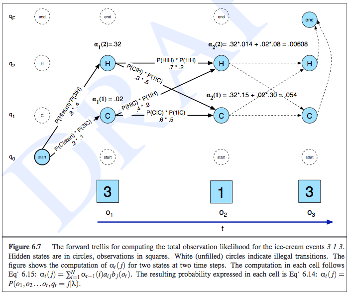
This example was about determining the observation likelihood of seeing three, one, and then three ice creams eaten in a day, and the state variables represented the temperature of the day. In the trellis, the rows correspond to the possible realizations of each state, along with one other row to symbolically represent the emission/observation/evidence. The notation of \(\alpha_t(j)\) represents the probability of the observation sequence and being at a particular state at time \(t\), so \(\alpha_t(j) = P(e_{1:t},x_t = j)\). The computation of \(\alpha\) is done recursively in an intuitive manner, as shown in the image:

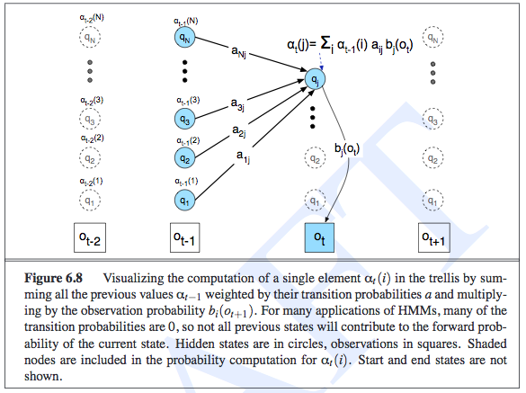
Intuitively, the likelihood of an observation sequence should be the sum of all the possible state sequences that could have led to that observation. The fact that we are summing up and storing probabilities in the previous \(\alpha_{t-1}\) terms is an indication of the HMM’s independence assumptions, and is what lets us do inference efficiently. Oh, and to actually compute the observations, we do need to sum out \(x_t\) from \(\alpha_t(j)\).

By the way, did you notice that these “updates” that we are doing are exactly what we did for the filtering step earlier? It’s just taking an earlier factor (representing whatever probability we want) and multiplying it by the transition and then the emission probability! In Russell and Norvig, the update equation is called \(z_{1:t+1} = {\rm FORWARD}(z_{1:t}, e_{t+1})\), and \(z_{1:t}\) can represent \(f_{1:t} = P(X_t \mid e_{1:t})\) or \(\ell_{1+t} = P(e_{1:t}, X_t)\). While \(f\) and \(\ell\) are clearly different, their updates are the same. And this FORWARD subroutine is what we generally mean when we talk about “the forward algorithm.”

The Viterbi Algorithm (Decoding)

This is another common inference task. Given a series of observations, the Viterbi algorithm helps us to determine the most likely sequence of states the system went to produce those observations. This is similar to the forward algorithm that we used to compute the likelihood of an observation sequence, but here we will now take max-es instead of summations, and we also have to keep a series of “backtrace pointers” so that we can reproduce our path.

Here’s the intuition: suppose we want to find the most likely path to some state \(X_t = x_t\). To do that, we need to find the most likely state path through \(X_{t-1}\), and then compare all the possible realizations of \(X_{t-1}\) along with the transition (and emission, but those are the same) probabilities going to the current \(X_t\) state. Then we pick the highest likelihood one, and add that particular \(x_{t-1}\) to the path (note the lowercase here!). Mathematically, we express it as follows:

The “messages” here are not forward messages but instead

The time and space complexity is linear in terms of the length of the sequence, \(t\), but for filtering, we don’t have the space taking up linear time since there are no backpointers.

Training the Parameters with EM

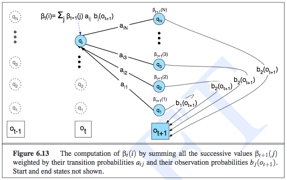
The purpose of the Baum-Welch algorithm (which is an example of the Expectation-Maximization algorithm), is to determine the parameters of an HMM given observed data. Somewhat confusingly, Jurafsky calls it the forward-backward algorithm. Russell calls the forward-backward algorithm as the algorithm that computes all the forward and backward probability messages defined earlier². But I guess they might be doing the same thing, because training HMMs will require us to compute the backward probabilities anyway. Jurafsky defines the backward probability to be exactly the same as what Russell defines it, i.e., as the probability of seeing the observations from time \(t+1\) to the end, given that we are at some state in time \(t\), or \(X_t\). The recursion of the backwards probability is shown in the following image, where we now see that we had to keep separate emission probabilities for each state, unlike in the forward probability case.

To estimate the parameters of the transition probability matrix, for a given element \(P(x_t \mid x_{t-1})\), we must count the expected proportion of times that the system undergoes a transition from state realization \(x_{t-1}\) to state realization \(x_t\). The expected counts are what EM computes, since those are the latent variables.

The following diagram shows the various things we have to compute to get the expected counts. Notice that the diagram is computing the probability of being in state \(i\) then state \(j\), jointly with the observation sequence. Thus, after this step, we would divide by \(P(e_{1:t})\) (or \(P(O \mid \lambda)\) in their notation). We then sum over all times, and that gives us the expected number of transitions from state \(i\) to state \(j\).

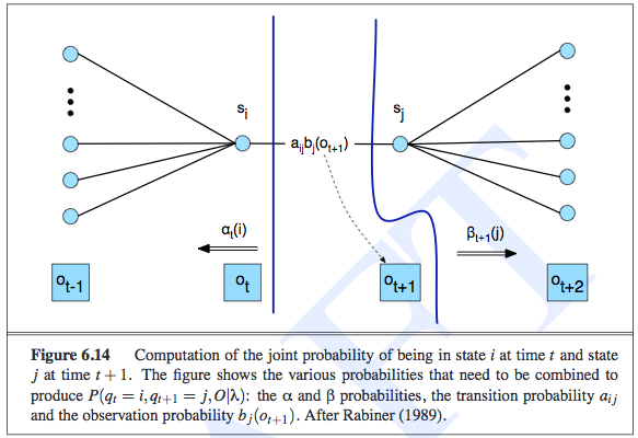
We follow a similar procedure for estimating the parameters of the emission probability.

The M-step is simple here; it turns expected counts into MLE for the corresponding parameters.

Particle Filtering

I got confused about particle filtering earlier. I assumed it broadly meant any algorithm that sampled something, but in fact, it has a specific meaning in the context of HMMs and Dynamic Bayesian Networks more generally. It is indeed a sampling algorithm, but has some interesting properties that are worth discussing in its own right.

First, when do we want to do particle filtering? We want to do this if exact inference in HMMs is intractable, or if the speed of sampling (and computing its corresponding probabilities) is more important than exact answers.

A naive way of performing exact inference in an HMM is to “unroll” it into a normal Bayesian Network. Technically, HMMs are infinitely long, so what we would do is chop off the HMM after the last time step that has a query or evidence variable, since by the structure of an HMM, anything after is not relevant to the query³. But if we did filtering after each observation, we would have to redo a lot of computations from the start \(X_0\) to the set of variables at the current time step. To save on memory costs, we realize that if we do filtering for a given time \(t+1\), we only need the relevant probability distribution from the previous time \(t\), since the computation is done recursively. Unfortunately, when we do this “summing out” process a-la variable elimination, that will iterate through the set of states, and this computation will grow exponentially due to the need to construct an exponentially large factor table⁴.

Thus, we need to use approximate inference methods. In a previous post, I discussed likelihood weighting, which is a sampling algorithm that we can adapt for the HMM setting. We do, however, have to ensure that we do not unroll the entire HMM, and we have to make sure our weights are not being driven to zero.

Likelihood weighting (just like rejection sampling) suffers as the number of evidence variables increases, because the weight of each sample is based on the product of all the \(P(E_i = e_i \mid E_{\pi_i})\) terms, which drives our values down to zero. But there is something that might be even worse than that. When we sample our non-evidence variables, ideally we would like those samples to depend on the evidence variables, so they can “guide” the sampling correctly. Unfortunately, if all the evidence variables tend to be downstream, i.e., they occur late in the variable ordering, then the sampling for the non-evidence variables will not depend on the evidence, even though the actual variables should depend on each other⁵. Sadly, in an HMM, all state variables have the property such that all the evidence relevant to them is downstream! (The ones before it are not downstream, but they are not ancestors either!)

What does particle filtering do, then, keeping in mind the weaknesses of likelihood weighting? Here is how the algorithm works. We initialize a population of \(N\) samples. The quantity \(N\) determines the time complexity of the algorithm, not the number of states. Then for each time step, we perform the following steps in sequence:

• We transition the samples according to the transition probabilities \(P(X_t \mid X_{t-1})\). This means we do not have to unroll the HMM.
• We then observe the evidence and downscale (i.e., multiply by a value in \([0,1]\)) each sample according to the evidence \(P(E_t \mid X_t)\). This is where the likelihood weighting “adaption” is obvious because now each sample is a fraction of a sample with some weight, and the overall distribution over the state variable’s realizations is the fraction of weights there divided by the total fraction of weights across all realizations.
• Then (and this is important), we resample to renormalize the distribution, where the resampling process is sampled according to the weights of the samples.

Here is a nice diagram from the CS 188 slides that suddenly clarified particle filtering for me.

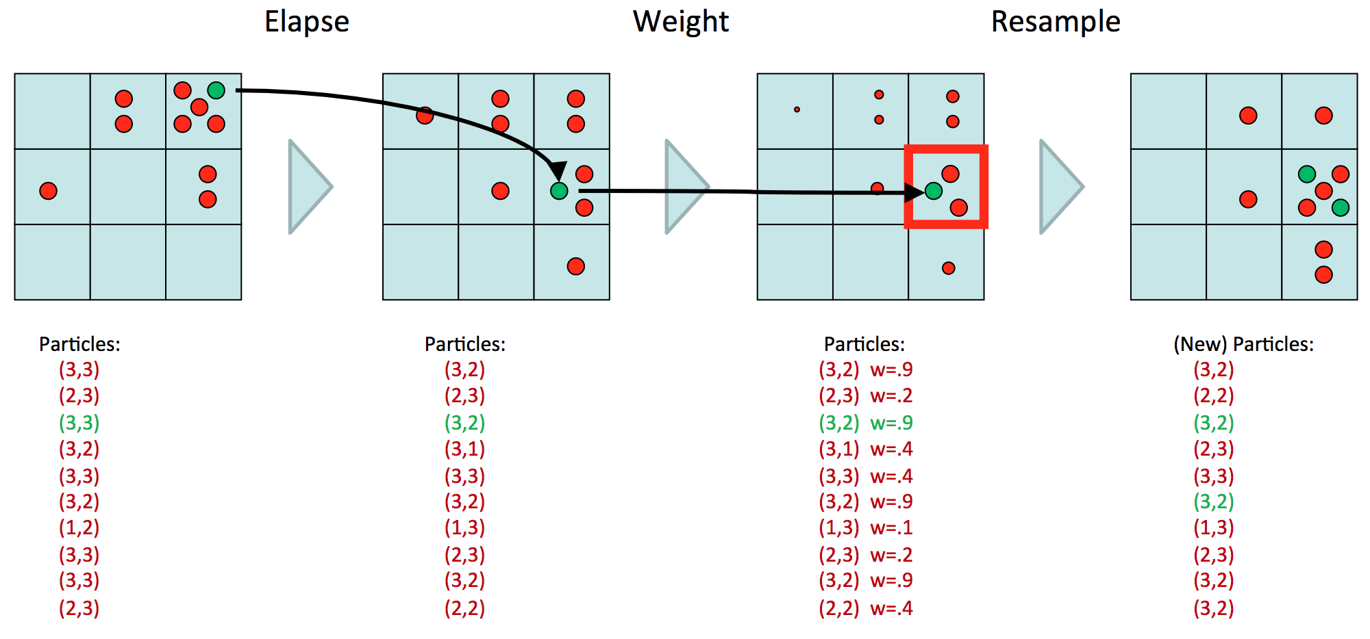
Here, we assume we have one state variable, with nine possible realizations. (Or we could have two state variables, each with three realizations, etc.) We have ten particles, representing our estimate of the distribution \(P(X_t \mid E_{1:t})\). Now the goal will be to determine the table of \(P(X_{t+1} \mid E_{1:t+1})\) values. First, we transition, which means we move each of the ten particles over to their next realization and multiply accordingly. Then, we observe \(E_{t+1} = e_{t+1}\), and downscale the values, resulting in points of different sizes, which are a diagram notation for weights. Above, we assume that whatever \(e_{t+1}\) was, the \(P(e_{t+1} \mid X_t)\) probability is high for that spot at coordinate \((3,2)\), and lower as we gradually go away from that spot. The last step is to resample, so we are resampling based on the probability distribution of the weighted samples. So we get five samples in that \((3,2)\) block because \(3(.9)\) divided by the sum of the weights (note: there’s a typo on the slides) gives a “high” probability. Note now that we have “normal-sized” samples again.

At this point, we should ask ourselves why we even bother resampling. It’s not completely clear to me, but it has to do with how we constantly rescale the weights downwards. In general, it’s not a good idea to have such small weights, because then the more evidence we have, the more likely we will just have a bunch of zero-probability particles. In other words, most particles end up in low-likelihood places in the state space. Still, I don’t quite buy some of the textbook explanations on this because couldn’t we just perform the computations in log space?