Independent Component Analysis — A Gentle Introduction

In this post, I give a brief introduction to independent component analysis (ICA), a machine learning algorithm useful for a certain niche of problems. It is not as general as, say, regression, which means many introductory machine learning courses won’t have time to teach ICA. I first describe the rationale and problem formulation. Then I discuss a common algorithm to solve ICA, courtesy of Bell and Sejnowski.

Motivation and Problem Formulation

Here’s a quick technical overview: the purpose of ICA is to explain some desired non-Gaussian data by figuring out a linear combination of statistically independent components. So what does that really mean?

This means we have some random variable — or more commonly, a random vector — that we observe, and which comes from a combination of different data sources. Consider the canonical cocktail party problem. Here, we have a group of people conversing at some party. There are two microphones stationed in different locations of the party room, and at time indices \(i = \{1, 2, \ldots \}\), the microphones provide us with voice measurements \(x_1^{(i)}\) and \(x_2^{(i)}\), such as amplitudes.

For simplicity, suppose that throughout the entire party, only two people are actually speaking, and that their speech signals are independent of each other (this is crucial). At time index \(i\), they speak with signals \(s_1^{(i)}\) and \(s_2^{(i)}\), respectively. But since the two people are in different locations of the room, the microphones each record signals from a different combination of the two people’s voices. The goal of ICA is, given the time series data from the microphones, to figure out the original speakers’ speech signals. The combination is assumed to be linear in that

for unknown coefficients \(a_{11},a_{12},a_{21},a_{22}\).

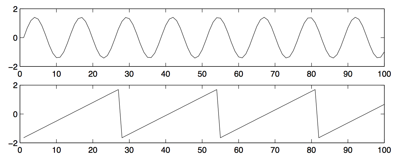
Here’s a graphical version, from a well-known ICA paper. The following image shows two (unrealistic) wavelength diagrams of two people’s voices:

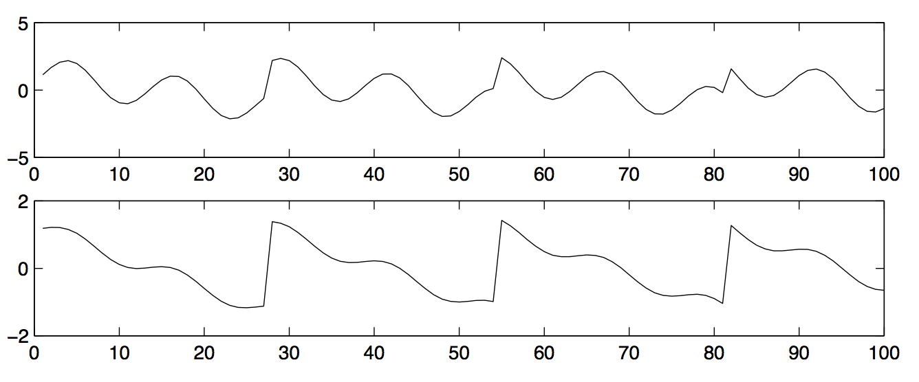
The data that is observed from the two microphones is in the following image:

The goal is to recover the original people’s wavelengths (i.e., the two graphs in the first of the two images I posted) when we are only given the observed data (i.e., the two graphs from the second image). Intuitively, it seems like the first observed wavelength must have come from a microphone closer to the first person, because its shape more closely matches person 1’s wavelength. The opposite is true for the second microphone.

More generally, consider having \(n\) microphones and \(n\) independent speakers; the numerical equality of microphones and speakers is for simplicity. In matrix form, we can express the ICA problem as \(x^{(i)} = As^{(i)}\) where \(A\) is an unknown, square, invertible mixing matrix that does not depend on the time interval. Like the assumptions regarding \(n\), the invertibility of \(A\) is to make our problem simple to start. We also know that all \(x^{(i)}\) and \(s^{(i)}\) are \(n\)-dimensional random vectors. The goal is to recover the unseen sources \(s^{(i)}\). To simplify the subsequent notation, I omit the \(i\) notation, but keep in mind that it’s there.

How does the linear combination part I mentioned earlier relate to this problem formulation? When we express problems in \(x = As\) form, that can be viewed as taking linear combinations of components of \(s\) along with the appropriate row of \(A\). For instance, the first component (remember, there are \(n\) of them) of the vector \(x\) is the dot product of the first row of \(A\) and the full vector \(s\). This is a linear combination of independent source signals \(s_1,s_2,\ldots,s_n\) with coefficients \(a_{11},a_{12}, \ldots, a_{1n}\) based on the first row of \(A\).

Before moving on to an algorithm that can recover the sources, consider the following insights:

1. What happens if we know \(A\)? Then multiply both sides of \(x = As\) by \(A^{-1}\) and we are done. Of course, the point is that we don’t know \(A\). It is what computer scientists call a set of latent variables. In fact, one perspective of our problem is that we need to get the optimal \(A^{-1}\) based on our data.
2. The following ambiguities regarding \(A\) will always hold: we cannot determine the variance of the components of \(s\) (due to scalars canceling out in \(A\)) and we also cannot determine ordering of \(s\) (due to permutation matrices). Fortunately, these two ambiguities are not problematic in practice¹.
3. One additional assumption that ICA needs is that the independent source components \(s_1, s_2, \ldots, s_n\) are not Gaussian random variables. If they are, then the rotational symmetry of Gaussians means we cannot distinguish among the distributions when analyzing their combinations. This requirement is the same as ensuring that the \(s\) vector is not multivariate Gaussian.

Surprisingly, as long as the source components are non-Gaussian, ICA will typically work well for a range of practical problems! Next, I’d like to discuss how we can “solve” ICA.

The Bell and Sejnowski ICA Algorithm

We describe a simple stochastic gradient descent algorithm to learn the parameter \(A^{-1}\) of the model. To simplify notation, let \(W = A^{-1}\) so that its rows can be denoted by \(w_i^\top\). Broadly, the goal is to figure out some way of determining the log-likelihood of the training data that depends on the parameter \(W\), and then perform updates to iteratively improve our estimated \(W\). This is how stochastic gradient descent typically works, and the normal case is to take logarithms to make numerical calculations easier to perform. Also, we will assume the data \(x_i\) are zero-mean, which is fine because we can normally “shift” a distribution to center it at 0.

For ICA, suppose we have \(m\) time stamps \(i = \{1, 2, \ldots, m\}\). The log-likelihood of the data is

where we note the following:

1. The determinant of \(W\) is denoted with single vertical bars surrounding it
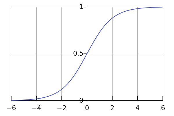
2. \(g'\) is the derivative of the sigmoid function \(g\) (not the sigmoid function itself!)

Let’s explain why this formula makes sense. It comes from taking logarithms of the density of \(x^{(i)}\) at each time stamp. Note that \(x = As\) so if we let \(p\) denote the density function of \(x^{(i)}\), then \(p(x^{(i)}) = |W| \prod_{j=1}^{n} p_j(w_j^\top x^{(i)})\), where \(p_j\) is the density of the individual source \(j\). We can split the product this way due to the independence among the sources, and the \(w_j\) terms are just (vector) constants so they can be separated as well. For a more detailed overview, see Andrew Ng’s lecture notes; in particular, we need the \(|W|\) term due to the effect of linear transformations.

Unfortunately, we don’t know the density of the individual sources, so we approximate them with some “good” density and make them equal to each other. We can do this by taking the derivative of the sigmoid function:

The reason why this works is that the sigmoid function satisfies the properties of a cumulative distribution function, and by differentiating such a function, we get a probability density function. And since it works well in practice (according to Andrew Ng), we might as well use it.

Great, so now that we have the log-likelihood equation, what is the stochastic gradient descent update rule? It is (remember that \(g\) is the sigmoid function):

where \(\alpha\) is the standard learning rate parameter, and the \(i\) that we pick for each iteration update varies (ideally sampling from the \(m\) training data pieces uniformly). Notice that the term in the parentheses is a matrix: we’re taking an outer product and then adding another matrix. To get that update rule from the log-likelihood equation, we take the gradient \(\nabla_W \ell(W)\), though I think we omit the first summation over \(m\) terms. Matrix calculus can be tricky and one of the best sources I found for learning about this is (surprise) another one of Andrew Ng’s lecture notes (look near the end). It took a while for me to verify but it should work as long as the \(m\) summation is omitted, i.e., we do this for a fixed \(x^{(i)}\). To find the correct outer product vectors to use, it may help to use the sigmoid’s nice property that \(g'(x) = g(x) (1-g(x))\). Lastly, don’t forget to take the logarithm into account when taking the derivatives.

There are whole books written on how to decide when to stop iterating, so I won’t get into that. Once it converges, perform \(s^{(i)} = Wx^{(i)}\) and we are done, assuming we just wanted the \(s\) vectors at all times (not always the case!).

Well, that’s independent component analysis. Remember that this is just one way to solve related problems, and it’s probably on the easier side.

References and Further Reading

1. Independent Component Analysis: Algorithms and Applications
2. Andrew Ng’s lecture notes