Gradient Descent Converges to Minimizers

The title of this blog post is the name of a preprint recently uploaded to arXiv by several researchers at Berkeley, including Ben Recht, who has taught two of my classes (so far). Judging by the arXiv comments, this paper is in submission to COLT 2016, so we won’t know about its acceptance until April 25. But it looks like quite a number of Berkeley people have skimmed this paper; there was some brief discussion about this on a robotics email list. Furthermore, there’s also been some related work about gradient descent, local minima, and saddle points in the context of neural networks. I’ve read two such papers: The Loss Surfaces of Multilayer Networks and Identifying and Attacking the Saddle Point Problem in High-Dimensional Non-convex Optimization. Consequently, I thought it would be interesting to take a look at the highlights of this paper.

Their main contribution is conveniently outlined in a single obvious paragraph (thank you for clear writing!!):

If \(f: \mathbb{R}^d \to \mathbb{R}\) is twice continuously differentiable and satisfies the strict saddle property, then gradient descent with a random initialization and sufficiently small constant step size converges to a local minimizer or negative infinity almost surely.

Let’s make it clear what this contribution means:

• We’re dealing with the gradient method, \(x_{k+1} = x_k - \alpha\nabla f(x_k)\). It’s nothing too fancy, and the constant step size makes the analysis easier.

• The sufficiently small step size means we want \(0 < \alpha < 1/L\) where \(L\) is the Lipschitz constant. In other words, it satisfies the well-known inequality \(\|\nabla f(x) - \nabla f(y)\|_2 \le L \|x-y\|_2\) for all \(x\) and \(y\). I have used this inequality a lot in EE 227C.

• The strict saddle property restricts \(f\) so that every critical point (i.e., those points \(x\) such that \(\nabla f(x) = 0\)) is either (a) a local minimizer, or (b) has \(\lambda_{\min}(\nabla^2f(x)) < 0\). It serves to restrict \(f\) because other functions could have critical points where all the eigenvalues are zero. Note that since the Hessian is a symmetric matrix, all the eigenvalues are real numbers. In addition, a local minimizing point \(x\) means the eigenvalues of \(\nabla^2f(x)\) are all strictly positive.

• They claim that the gradient method will go to a local minimizer. But where else could it go to? There are two other options: saddle points, and local maxima. Gradient descent, however, cannot go to local maxima because it is by definition a descent procedure, unless (I think) for some reason we’ve initialized \(x_0\) as a point that is already a global maxima, so \(\nabla f(x_0) = 0\) and we get nowhere. So the only thing we worry about are saddle points. Thus, if “saddle points are not a problem” as suggested in the paper, then that therefore means gradient descent converges to local minimizers, as desired.

It’s worth discussing saddle points in more detail. The paper “Identifying and Attacking…” uses the following diagrams to provide intuition:

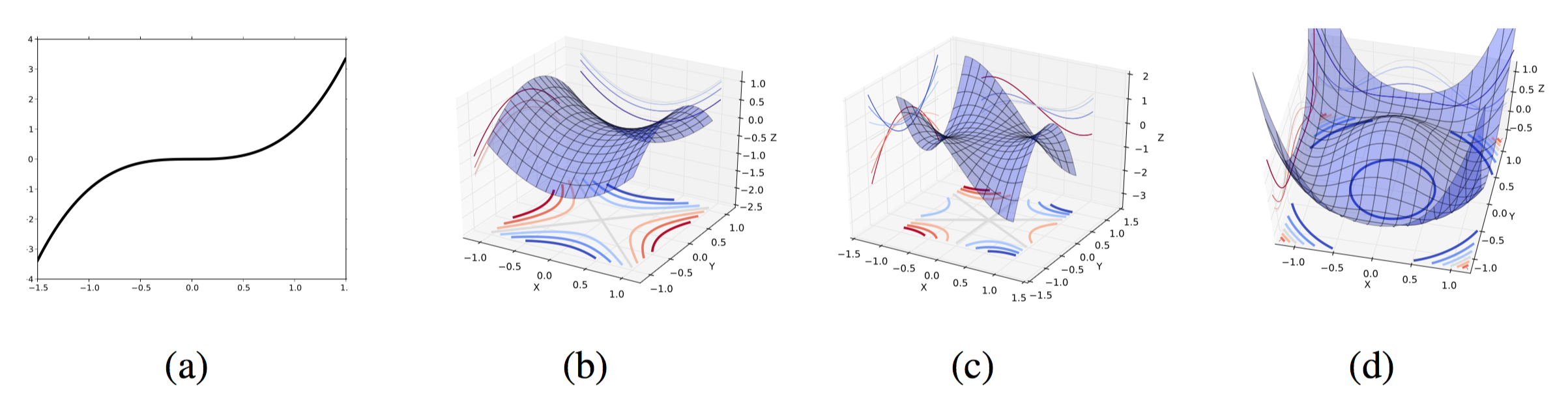
Image (a) is a saddle point of a 1-D (i.e., scalar) function. Images (b) and (c) represent saddle points in higher dimensions. They are characterized by the eigenvalues of the Hessian at those critical points. If all eigenvalues are non-zero and either strictly positive or strictly negative, then we get the shape of (b) with a min-max structure. If there exists a zero eigenvalue, then we get (c) with a degenerate Hessian. (Recall that a matrix is invertible if and only if all its eigenvalues are non-zero.) Image (d) is a weird “gutter shape” which also results from at least one zero eigenvalue. I’m not completely sure I buy their explanation – I’d need a little more explanation for why this happens. But I suppose the point is that the authors of “Gradient Descent Converges to Minimizers” don’t want to consider degenerate cases with zero eigenvalues. It must make the analysis easier.

Section 3 of “Gradient Descent Converges to Minimizers” provides two examples for intuition. The first example is \(f(x) = \frac{1}{2}x^THx\), where \(H={\rm diag}(\lambda_1, \lambda_2, \ldots, \lambda_n)\) and has no zero components (and hence no zero eigenvalues) but it must have at least one positive and at least one negative component. Otherwise, we wouldn’t have any saddle points! By the way, the only critical point for this function is \(x=0\), as \(\nabla f(x) = Hx=0\) if and only if \(x=0\).

The gradient update is \(x_{k+1} = (I-\alpha H)x_k\). Applying this recursively, we get \(x_{k+1} = (I-\alpha H)^{k+1}x_0\). More specifically, the iterates take on the following form:

Indeed, an analysis of gradient descent with \(0 < \alpha < 1/L\) shows that gradient descent will only converge to \(x=0\) if the initial point \(x_0\) is in the span of \(\{e_1, \ldots, e_k\}\) where \(k\) represents the number of strictly positive eigenvalues (so \(k < n\)). Remember: we don’t actually want to converge to that point, since it is a saddle point! But fortunately, as \(k < n\), if we randomly initialize \(x_0\) appropriately, the only way our iterates converge to the zero vector is if all components from \(k+1\) to \(n\) were exactly zero, and the probability of that happening is zero. Great! We don’t converge to the (bad) critical point! We converge to … a better point, I hope. (The paper uses the term “diverge” but I get uneasy reading that.)

The second example is \(f(x,y) = \frac{1}{2}x^2 + \frac{1}{4}y^4 - \frac{1}{2}y^2\). Finding the explicit gradient update is straightforward, and is provided in the paper. They also explicitly state the three critical points of \(f\). Their argument is similar to the previous example in that they can reduce the cases of converging to an undesirable saddle point to a case which would require initializing a certain component of the starting 2-D point \((x_0,y_0)\) to zero, which cannot happen with random initialization (well, the technical way to say that is “zero measure” …).

I still have a few burning questions on these (plus some of the other stuff mentioned in Section 3) but I’ll hold off on writing about those once I have time to get to the meat of this paper, Section

1. In the meantime, it will be interesting to see what kind of work gets built off of this one.