Going Deeper Into Reinforcement Learning: Understanding Q-Learning and Linear Function Approximation

As I mentioned in my review on Berkeley’s Deep Reinforcement Learning class, I have been wanting to write more about reinforcement learning, so in this post, I will provide some comments on Q-Learning and Linear Function Approximation. I’m hoping these posts can serve as another set of brief RL introductions, similar to Andrej’s excellent post on deep RL.

Last year, I wrote an earlier post on the basics of MDPs and RL. This current one serves as the continuation of that by discussing how to scale RL into settings that are more complicated than simple tabular scenarios but nowhere near as challenging as, say, learning how to play Atari games from high-dimensional input. I won’t spend too much time trying to labor though the topics in this post, though. I want to save my effort for the deep variety, which is all the rage nowadays and a topic which I hope to eventually write a lot about for this blog.

To hep write this post, here are two references I used to quickly review Q-Learning with function approximation.

1. Tutorial on RL and Linear Function Approximators
2. Barto and Sutton’s RL book, in HTML

I read (1) entirely, and (2) only partly, since it is, after all, a full book (note that the authors are in the process of making a newer edition!). Now let’s move on to discuss an important concept: value iteration with function approximation.

Value Iteration with Function Approximation

Value Iteration is probably the first RL-associated algorithm that students learn. It lets us assign values \(V(s)\) to states \(s\), which can then be used to determine optimal policies. I explained the algorithm in my earlier post, but just to be explicit, here’s a slide from my CS 287 class last fall which describes the procedure:

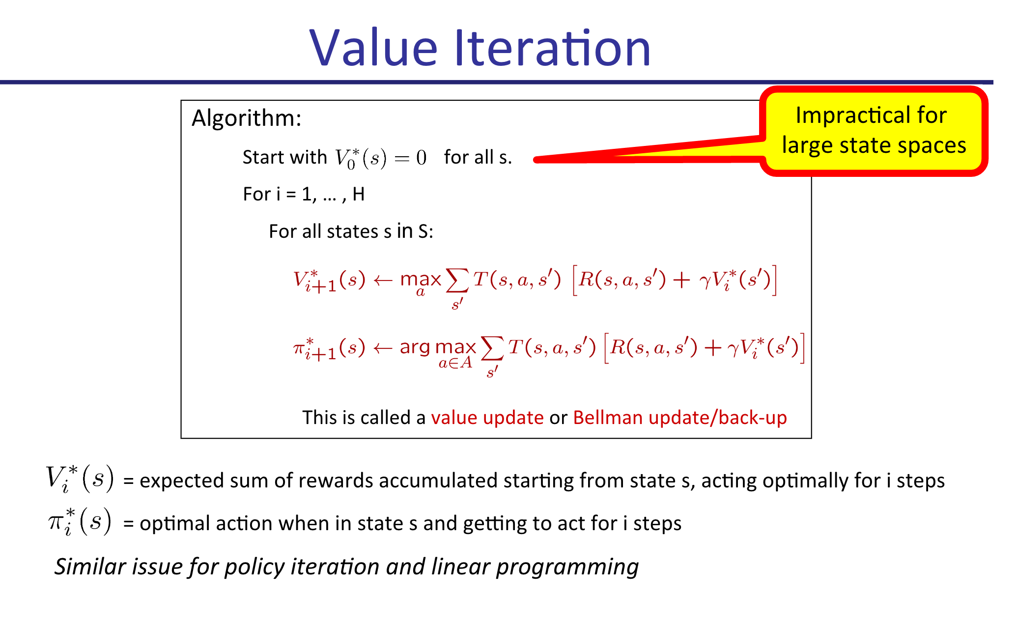
Looks pretty simple, right? For each iteration, we perform updates on our values \(V_{i}^*\) until convergence. Each iteration, we can also update the policy \(\pi_i^*\) for each state, if desired, but this is not the crucial part of the algorithm. In fact, since the policy updates don’t impact the \(V_{i+1}^*(s)\) max-operations in the algorithm (as shown above), we can forget about updating \(\pi\) and do that just once after the algorithm has converged. This is what Barto and Sutton do in their Value Iteration description.

Unfortunately, as suggested by the slide, (tabular) Value Iteration this is not something we can do in practice beyond the simplest of scenarios due to the curse of dimensionality in \(s\). Note that \(a\) is not usually a problem. Think of \(9 \times 9\) Go, for instance: according to reference (1) above, there are \(|\mathcal{S}| = 10^{38}\) states, but just \(|\mathcal{A}| = 81\) actions to play. In Atari games, the disparity is even greater, with far more states but perhaps just two to five actions per game.

The solution is to obtain features and then represent states with a simple function of those features. We might use a linear function, meaning that

where \(\theta_0\) is a bias term with 1 “absorbed” into \(\phi\) for simplicity. This function approximation dramatically reduces the size of our state space from \(|\mathcal{S}|\) into “\(|\Theta|\)” where \(\Theta\) is the domain for \(\theta \in \mathbb{R}^n\). Rather than determining \(V_{i+1}^*(s)\) for all \(s\), each iteration our goal is to instead update the weights \(\theta_i\).

How do we do that? The most straightforward way is to reformulate it as a supervised learning problem. From the tabular version above, we know that the weights should satisfy the Bellman optimality conditions. We can’t use all the states for this update, but perhaps we can use a small subset of them?

This motivates the following algorithm: each iteration \(i\) in our algorithm with current weight vector \(\theta^{(i)}\), we sample a very small subset of the states \(S' \subset S\) and compute the official one-step Bellman backup updates:

Then we find the next set of weights:

which can be done using standard supervised learning techniques. This is, in fact, an example of stochastic gradient descent.

Before moving on, it’s worth mentioning the obvious: the performance of Value Iteration with function approximation is going to depend almost entirely on the quality of the features (along with the function representation, i.e. linear, neural network, etc.). If you’re programming an AI to play PacMan, the states \(s\) will be the game board, which is far too high-dimensional for tabular representations. Features will ideally represent something relevant to PacMan’s performance in the game, such as the distance to the nearest ghost, the distance to the nearest pellet, whether PacMan is trapped, and so on. Don’t neglect the art and engineering of feature selection!

Q-Learning with Function Approximation

Value Iteration with function approximation is nice, but as I mentioned in my last post, what we really want in practice are \(Q(s,a)\) values, due to the key fact that

which avoids a costly sum over the states. This will cost us extra in the sense that we have to now use a function with respect to \(a\) in addition to \(s\), but again, this is not usually a problem since the set of actions is typically much smaller than the set of states.

To use Q-values with function approximation, we need to find features that are functions of states and actions. This means in the linear function regime, we have

What’s tricky about this, however, is that it’s usually a lot easier to reason about features that are only functions of the states. Think of the PacMan example from earlier: it’s relatively easy to think about features by just looking at what’s on the game grid, but it’s harder to wonder about what happens to the value of a state assuming that action \(a\) is taking place.

For this reason, I tend to use the following “dimension scaling trick” as recommended by reference (1) above, which makes the distinction between different actions explicit. To make this clear, image an MDP with two features and four actions. The features for state-action pair \((s,a_i)\) can be encoded as:

Why the need to use different feature for different actions? Intuitively, if we didn’t do this (and kept \(\phi(s,a)\) with just two non-bias features) then the action would have no effect! But actions do have impacts on the game. To use the PacMan example again, imagine that the PacMan agent has a pellet to its left, so the agent is one move away from being invincible. At the same time, however, there could be a ghost to PacMan’s right! The action that PacMan takes in that state (LEFT or RIGHT) will have a dramatic impact on the resulting reward obtained! It is therefore important to take the actions into account when featurizing Q-values.

As a reminder before moving on, don’t forget the bias term! They are necessary to properly scale the function values independently of the features.

Online Least Squares Justification for Q-Learning

I now want to sketch the derivation for Q-Learning updates to provide intuition for why it works. Knowing this is also important to understand how the training process works for the more advanced Deep-Q-Network algorithm/architecture.

Recall the standard Q-Learning update without function approximation:

Why does this work? Imagine that you have some weight vector \(\theta^{(i)}\) at iteration \(i\) of the algorithm and you want to figure out how to update it. The standard way to do so is with stochastic gradient descent, as mentioned earlier in the Value Iteration case. But what is the loss function here? We need that so we can compute the gradient.

In Q-Learning, when we approximate a state-action value \(Q(s,a)\), we want it to be equal to the reward obtained, plus the (appropriately discounted) value of playing optimally from thereafter. Denote this “target” value as \(Q^+(s,a)\). In the tabular version, we set the target as

It is infeasible to sum over all states, but we can get a minibatch estimate of this by simply considering the samples we get: \(Q^+(s,a) \approx R(s,a,s') + \gamma \max_{a'}Q^+(s',a')\). Averaged over the entire run, these will average out to the true value.

Assuming we’re in the function approximation case (though this is not actually needed), and that our estimate of the target is \(Q(s,a)\), we can therefore define our loss as:

Thus, our gradient update procedure with step size \(\alpha\) is

This is how we update the weights for Q-Learning. Notice that \(\theta^{(i)}\) and \(\phi(s,a)\) are vectors, while \(Q^+(s,a)\) is a scalar.

Concluding Thoughts

Well, there you have it. We covered:

• Value Iteration with (linear) function approximation, a relatively easy-to-understand algorithm that should serve as your first choice if you need to scale up tabular value iteration for a simple reinforcement learning problem.
• Q-Learning with (linear) function approximation, which approximates \(Q(s,a)\) values with a linear function, i.e. \(Q(s,a) \approx \theta^T\phi(s,a)\). From my experience, I prefer to use the states-only formulation \(\theta^T\phi(s)\), and then to apply the “dimension scaling trick” from above to make Q-Learning work in practice.
• Q-Learning as a consequence of online least squares, which provides a more rigorous rationale for why it makes sense, rather than relying on hand-waving arguments.

The scalability benefit of Q-Learning (or Value Iteration) with linear function approximation may sound great over the tabular versions, but here is the critical question: is a linear function approximator appropriate for the problem?

This is important because a lot of current research on reinforcement learning is applied towards complicated and high dimensional data. A great example, and probably the most popular one, is learning how to play Atari games from raw (210,160,3)-dimensional arrays. A linear function is simply not effective at learning \(Q(s,a)\) values for these problems, because the problems are inherently non-linear! A further discussion of this is out of the scope of this post, but if you are interested, Andrew Ng addressed this in his talk at the Bay Area Deep Learning School a month ago. Kevin Zakka has a nice blog post which summarizes Ng’s talk.¹ In the small data regime, many algorithms can achieve “good” performance, with differences arising in large part due to who tuned his/her algorithm the most, but in the high-dimensional big-data regime, the complexity of the model matters. Neural networks can learn and represent far more complicated functions.

Therefore, in my next post, I will introduce and discuss Q-Learning with neural networks as the function approximation. It will use the Atari games as a running example. Stay tuned!