Understanding Higher Order Local Gradient Computation for Backpropagation in Deep Neural Networks
Introduction
One of the major difficulties in understanding how neural networks work is due to the backpropagation algorithm. There are endless texts and online guides on backpropagation, but most are useless. I read several explanations of backpropagation when I learned about it from 2013 to 2014, but I never felt like I really understood it until I took/TA-ed the Deep Neural Networks class at Berkeley, based on the excellent Stanford CS 231n course.
The course notes from CS 231n include a tutorial on how to compute gradients for local nodes in computational graphs, which I think is key to understanding backpropagation. However, the notes are mostly for the one-dimensional case, and their main advice for extending gradient computation to the vector or matrix case is to keep track of dimensions. That’s perfectly fine, and in fact that was how I managed to get through the second CS 231n assignment.
But this felt unsatisfying.
For some of the harder gradient computations, I had to test several different ideas before passing the gradient checker, and sometimes I wasn’t even sure why my code worked! Thus, the purpose of this post is to make sure I deeply understand how gradient computation works.
Note: I’ve had this post in draft stage for a long time. However, I just found out that the notes from CS 231n have been updated with a guide from Erik Learned-Miller on taking matrix/vector derivatives. That’s worth checking out, but fortunately, the content I provide here is mostly distinct from his material.
The Basics: Computational Graphs in One Dimension
I won’t belabor the details on one-dimensional graphs since I assume the reader has read the corresponding Stanford CS 231n guide. Another nice post is from Chris Olah’s excellent blog. For my own benefit, I reviewed derivatives on computational graphs by going through the CS 231n example with sigmoids (but with the sigmoid computation spread out among finer-grained operations). You can see my hand-written computations in the following image. Sorry, I have absolutely no skill in getting this up quickly using tikz, Inkscape, or other visualization tactics/software. Feel free to right-click and open the image in a new tab. Warning: it’s big. (But I have to say, the iPhone7 plus makes really nice images. I remember the good old days when we had to take our cameras to CVS to get them developed…)
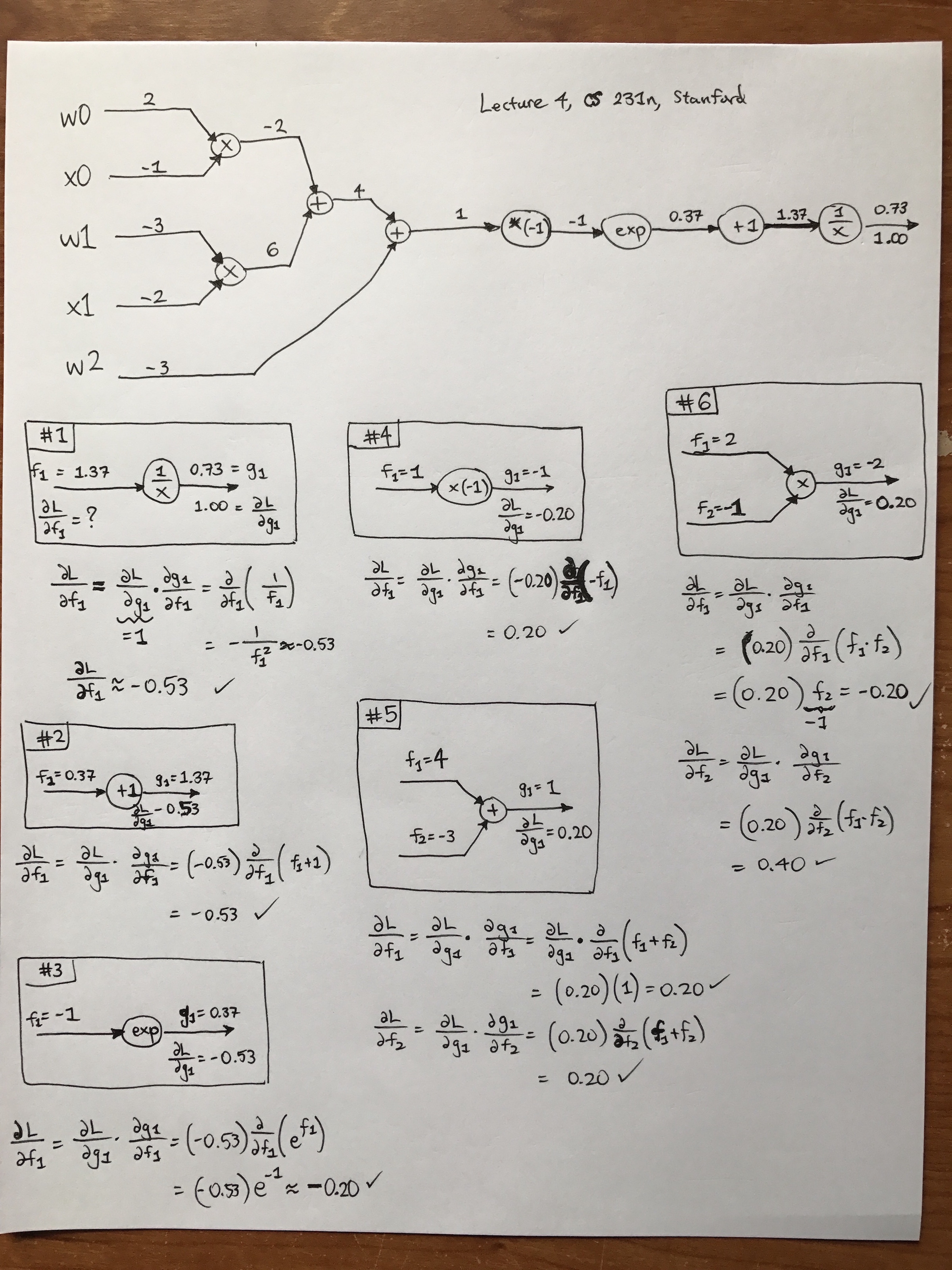
Another note: from the image, you can see that this is from the fourth lecture of CS 231n class. I watched that video on YouTube, which is excellent and of high-quality. Fortunately, there are also automatic captions which are highly accurate. (There’s an archived reddit thread discussing how Andrej Karpathy had to take down the videos due to a related lawsuit I blogged about earlier, but I can see them just fine. Did they get back up somehow? I’ll write more about this at a later date.)
When I was going through the math here, I came up with several rules to myself:
-
There’s a lot of notation that can get confusing, so for simplicity, I always denoted inputs as \(f_1,f_2,\ldots\) and outputs as \(g_1,g_2,\ldots\), though in this example, we only have one output at each step. By doing this, I can view the \(g_1\)s as a function of the \(f_i\) terms, so the local gradient turns into \(\frac{\partial g_1}{\partial f_i}\) and then I can substitute \(g_1\) in terms of the inputs.
-
When doing backpropgation, I analyzed it node-by-node, and the boxes I drew in my image contain a number which indicates the order I evaluated them. (I skipped a few repeat blocks just as the lecture did.) Note that when filling in my boxes, I only used the node and any incoming/outgoing arrows. Also, the \(f_i\) and \(g_i\) keep getting repeated, i.e. the next step will have \(g_i\) equal to whatever the \(f_i\) was in the previous block.
-
Always remember that when we have arrows here, the part above the arrow contains the value of \(f_i\) (respectively, \(g_i\)) and below the arrow we have \(\frac{\partial L}{\partial f_i}\) (respectively \(\frac{\partial L}{\partial g_i}\)).
Hopefully this will be helpful to beginners using computational graphs.
Vector/Matrix/Tensor Derivatives, With Examples
Now let’s get to the big guns — vectors/matrices/tensors. Vectors are a special case of matrices, which are a special case of tensors, the most generalized \(n\)-dimensional array. For this section, I will continue using the “partial derivative” notation \(\frac{\partial}{\partial x}\) to represent any derivative form (scalar, vector, or matrix).
ReLU
Our first example will be with ReLUs, because that was covered a bit in the
CS 231n lecture. Let’s suppose \(x \in \mathbb{R}^3\), a 3-D column vector
representing some data from a hidden layer deep into the network. The ReLU
operation’s forward pass is extremely simple: \(y = \max\{0,x\}\), which can be
vectorized using np.max.
The backward pass is where things get tricky. The input is a 3-D vector, and so is the output! Hence, taking the derivative of the function \(y(x): \mathbb{R}^3\to \mathbb{R}^3\) means we have to consider the effect of every \(x_i\) on every \(y_j\). The only way that’s possible is to use Jacobians. Using the example here, denoting the derivative as \(\frac{\partial y}{\partial x}\) where \(y(x)\) is a function of \(x\), we have:
\[\begin{align*} \frac{\partial y}{\partial x} &= \begin{bmatrix} \frac{\partial y_1}{\partial x_1} &\frac{\partial y_1}{\partial x_2} & \frac{\partial y_1}{\partial x_3}\\ \frac{\partial y_2}{\partial x_1} &\frac{\partial y_2}{\partial x_2} & \frac{\partial y_2}{\partial x_3}\\ \frac{\partial y_3}{\partial x_1} &\frac{\partial y_3}{\partial x_2} & \frac{\partial y_3}{\partial x_3} \end{bmatrix}\\ &= \begin{bmatrix} \frac{\partial}{\partial x_1}\max\{0,x_1\} &\frac{\partial}{\partial x_2}\max\{0,x_1\} & \frac{\partial}{\partial x_3}\max\{0,x_1\}\\ \frac{\partial}{\partial x_1}\max\{0,x_2\} &\frac{\partial}{\partial x_2}\max\{0,x_2\} & \frac{\partial}{\partial x_3}\max\{0,x_2\}\\ \frac{\partial}{\partial x_1}\max\{0,x_3\} &\frac{\partial}{\partial x_2}\max\{0,x_3\} & \frac{\partial}{\partial x_3}\max\{0,x_3\} \end{bmatrix}\\ &= \begin{bmatrix} 1\{x_1>0\} & 0 & 0 \\ 0 & 1\{x_2>0\} & 0 \\ 0 & 0 & 1\{x_3>0\} \end{bmatrix} \end{align*}\]The most interesting part of this happens when we expand the Jacobian and see that we have a bunch of derivatives, but they all evaluate to zero on the off-diagonal. After all, the effect (i.e. derivative) of \(x_2\) will be zero for the function \(\max\{0,x_3\}\). The diagonal term is only slightly more complicated: an indicator function (which evaluates to either 0 or 1) depending on the outcome of the ReLU. This means we have to cache the result of the forward pass, which easy to do in the CS 231n assignments.
How does this get combined into the incoming (i.e. “upstream”) gradient, which is a vector \(\frac{\partial L}{\partial y}\). We perform a matrix times vector operation with that and our Jacobian from above. Thus, the overall gradient we have for \(x\) with respect to the loss function, which is what we wanted all along, is:
\[\frac{\partial L}{\partial x} = \begin{bmatrix} 1\{x_1>0\} & 0 & 0 \\ 0 & 1\{x_2>0\} & 0 \\ 0 & 0 & 1\{x_3>0\} \end{bmatrix} \cdot \frac{\partial L}{\partial y}\]This is as simple as doing mask * y_grad where mask is a numpy array with 0s
and 1s depending on the value of the indicator functions, and y_grad is the
upstream derivative/gradient. In other words, we can completely bypass the
Jacobian computation in our Python code! Another option is to use y_grad[x <=
0] = 0, where x is the data that was passed in the forward pass (just before
ReLU was applied). In numpy, this will set all indices to which the condition x
<= 0 is true to have zero value, precisely clearing out the gradients where we
need it cleared.
In practice, we tend to use mini-batches of data, so instead of a single \(x
\in \mathbb{R}^3\), we have a matrix \(X \in \mathbb{R}^{3 \times n}\) with
\(n\) columns.1 Denote the \(i\)th column as \(x^{(i)}\). Writing out
the full Jacobian is too cumbersome in this case, but to visualize it, think of
having \(n=2\) and then stacking the two samples \(x^{(1)},x^{(2)}\) into a
six-dimensional vector. Do the same for the output \(y^{(1)},y^{(2)}\). The
Jacobian turns out to again be a diagonal matrix, particularly because the
derivative of \(x^{(i)}\) on the output \(y^{(j)}\) is zero for \(i \ne j\).
Thus, we can again use a simple masking, element-wise multiply on the upstream
gradient to compute the local gradient of \(x\) w.r.t. \(y\). In our code we
don’t have to do any “stacking/destacking”; we can actually use the exact same
code mask * y_grad with both of these being 2-D numpy arrays (i.e. matrices)
rather than 1-D numpy arrays. The case is similar for larger minibatch sizes
using \(n>2\) samples.
Remark: this process of computing derivatives will be similar to other activation functions because they are elementwise operations.
Affine Layer (Fully Connected), Biases
Now let’s discuss a layer which isn’t elementwise: the fully connected layer operation \(WX+b\). How do we compute gradients? To start, let’s consider one 3-D element \(x\) so that our operation is
\[\begin{bmatrix} W_{11} & W_{12} & W_{13} \\ W_{21} & W_{22} & W_{23} \end{bmatrix} \begin{bmatrix} x_1 \\ x_2 \\ x_3 \end{bmatrix} + \begin{bmatrix} b_1 \\ b_2 \end{bmatrix} = \begin{bmatrix} y_1 \\ y_2 \end{bmatrix}\]According to the chain rule, the local gradient with respect to \(b\) is
\[\frac{\partial L}{\partial b} = \underbrace{\frac{\partial y}{\partial b}}_{2\times 2} \cdot \underbrace{\frac{\partial L}{\partial y}}_{2\times 1}\]Since we’re doing backpropagation, we can assume the upstream derivative is given, so we only need to compute the \(2\times 2\) Jacobian. To do so, observe that
\[\frac{\partial y_1}{\partial b_1} = \frac{\partial}{\partial b_1} (W_{11}x_1+W_{12}x_2+W_{13}x_3+b_1) = 1\]and a similar case happens for the second component. The off-diagonal terms are zero in the Jacobian since \(b_i\) has no effect on \(y_j\) for \(i\ne j\). Hence, the local derivative is
\[\frac{\partial L}{\partial b} = \begin{bmatrix} 1 & 0 \\ 0 & 1 \end{bmatrix} \cdot \frac{\partial L}{\partial y} = \frac{\partial L}{\partial y}\]That’s pretty nice — all we need to do is copy the upstream derivative. No additional work necessary!
Now let’s get more realistic. How do we extend this when \(X\) is a matrix? Let’s continue the same notation as we did in the ReLU case, so that our columns are \(x^{(i)}\) for \(i=\{1,2,\ldots,n\}\). Thus, we have:
\[\begin{bmatrix} W_{11} & W_{12} & W_{13} \\ W_{21} & W_{22} & W_{23} \end{bmatrix} \begin{bmatrix} x_1^{(1)} & \cdots & x_1^{(n)} \\ x_2^{(1)} & \cdots & x_2^{(n)} \\ x_3^{(1)} & \cdots & x_3^{(n)} \end{bmatrix} + \begin{bmatrix} b_1 & \cdots & b_1 \\ b_2 & \cdots & b_2 \end{bmatrix} = \begin{bmatrix} y_1^{(1)} & \cdots & y_1^{(n)} \\ y_2^{(1)} & \cdots & y_2^{(n)} \end{bmatrix}\]Remark: crucially, notice that the elements of \(b\) are repeated across columns.
How do we compute the local derivative? We can try writing out the derivative rule as we did before:
\[\frac{\partial L}{\partial b} = \frac{\partial y}{\partial b} \cdot \frac{\partial L}{\partial y}\]but the problem is that this isn’t matrix multiplication. Here, \(y\) is a function from \(\mathbb{R}^2\) to \(\mathbb{R}^{2\times n}\), and to evaluate the derivative, it seems like we would need a 3-D matrix for full generality.
Fortunately, there’s an easier way with computational graphs. If you draw out the computational graph and create nodes for \(Wx^{(1)}, \ldots, Wx^{(n)}\), you see that you have to write \(n\) plus nodes to get the output, each of which takes in one of these \(Wx^{(i)}\) terms along with adding \(b\). Then this produces \(y^{(i)}\). See my hand-drawn diagram:
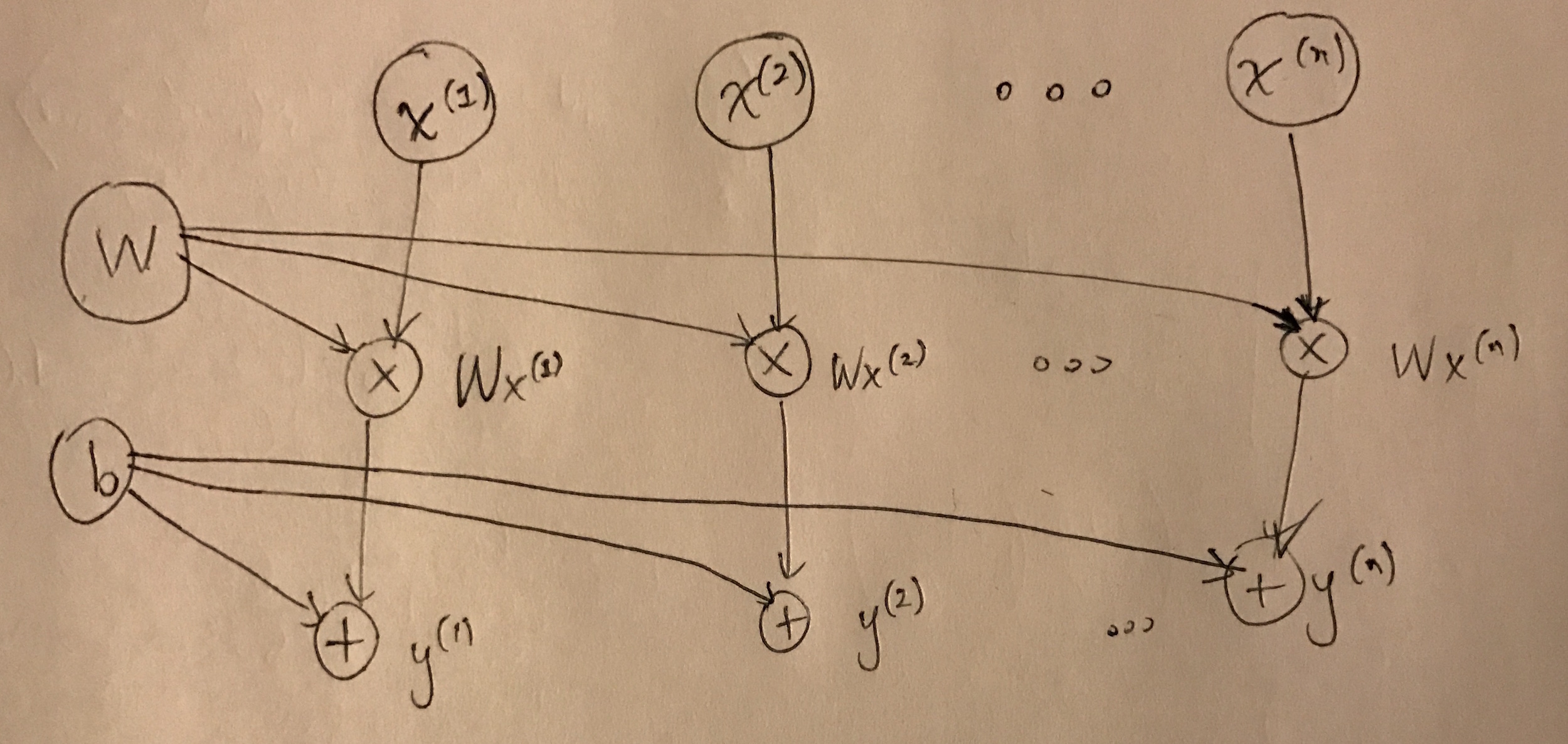
This captures the key property of independence among the samples in \(X\). To compute the local gradients for \(b\), it therefore suffices to compute the local gradients for each of the \(y^{(i)}\) and then add them together. (The rule in computational graphs is to add incoming derivatives, which can be verified by looking at trivial 1-D examples.) The gradient is
\[\frac{\partial L}{\partial b} = \sum_{i=1}^n \frac{\partial y^{(i)}}{\partial b} \frac{\partial L}{\partial y^{(i)}} = \sum_{i=1}^n \frac{\partial L}{\partial y^{(i)}}\]See what happened? This immediately reduced to the same case we had earlier,
with a \(2\times 2\) Jacobian being multiplied by a \(2\times 1\) upstream
derivative. All of the Jacobians turn out to be the identity, meaning that the
final derivative \(\frac{\partial L}{\partial b}\) is the sum of the columns of
the original upstream derivative matrix \(Y\). As a sanity check, this is a
\((2\times 1)\)-dimensional vector, as desired. In numpy, one can do this with
something similar to np.sum(Y_grad), though you’ll probably need the axis
argument to make sure the sum is across the appropriate dimension.
Affine Layer (Fully Connected), Weight Matrix
Going from biases, which are represented by vectors, to weights, which are represented by matrices, brings some extra difficulty due to that extra dimension.
Let’s focus on the case with one sample \(x^{(1)}\). For the derivative with respect to \(W\), we can ignore \(b\) since the multivariate chain rule states that the expression \(y^{(1)}=Wx^{(1)}+b\) differentiated with respect to \(W\) causes \(b\) to disappear, just like in the scalar case.
The harder part is dealing with the chain rule for the \(Wx^{(1)}\) expression, because we can’t write the expression “\(\frac{\partial}{\partial W} Wx^{(1)}\)”. The function \(Wx^{(1)}\) is a vector, and the variable we’re differentiating here is a matrix. Thus, we’d again need a 3-D like matrix to contain the derivatives.
Fortunately, there’s an easier way with the chain rule. We can still use the rule, except we have to sum over the intermediate components, as specified by the chain rule for higher dimensions; see the Wikipedia article for more details and justification. Our “intermediate component” here is the \(y^{(1)}\) vector, which has two components. We therefore have:
\[\begin{align} \frac{\partial L}{\partial W} &= \sum_{i=1}^2 \frac{\partial L}{\partial y_i^{(1)}} \frac{\partial y_i^{(1)}}{\partial W} \\ &= \frac{\partial L}{\partial y_1^{(1)}}\begin{bmatrix}x_1^{(1)}&x_2^{(1)}&x_3^{(1)}\\0&0&0\end{bmatrix} + \frac{\partial L}{\partial y_2^{(1)}}\begin{bmatrix}0&0&0\\x_1^{(1)}&x_2^{(1)}&x_3^{(1)}\end{bmatrix} \\ &= \begin{bmatrix} \frac{\partial L}{\partial y_1^{(1)}}x_1^{(1)} & \frac{\partial L}{\partial y_1^{(1)}} x_2^{(1)}& \frac{\partial L}{\partial y_1^{(1)}} x_3^{(1)}\\ \frac{\partial L}{\partial y_2^{(1)}} x_1^{(1)}& \frac{\partial L}{\partial y_2^{(1)}} x_2^{(1)}& \frac{\partial L}{\partial y_2^{(1)}} x_3^{(1)}\end{bmatrix} \\ &= \begin{bmatrix} \frac{\partial L}{\partial y_1^{(1)}} \\ \frac{\partial L}{\partial y_2^{(1)}}\end{bmatrix} \begin{bmatrix} x_1^{(1)} & x_2^{(1)} & x_3^{(1)}\end{bmatrix}. \end{align}\]We fortunately see that it simplifies to a simple matrix product! This seems to suggest the following rule: try to simplify any expressions to straightforward Jacobians, gradients, or scalar derivatives, and sum over as needed. Above, splitting the components of \(y^{(1)}\) allowed us to utilize the derivative \(\frac{\partial y_i^{(1)}}{\partial W}\) since \(y_i^{(1)}\) is now a real-valued function, thus enabling straightforward gradient derivations. It also meant the upstream derivative could be analyzed component-by-component, making our lives easier.
A similar case holds for when we have multiple columns \(x^{(i)}\) in \(X\). We would have another sum above, over the columns, but fortunately this can be re-written as matrix multiplication.
Convolutional Layers
How do we compute the convolutional layer gradients? That’s pretty complicated so I’ll leave that as an exercise for the reader. For now.
-
In fact, \(X\) is in general a tensor. Sophisticated software packages will generalize \(X\) to be tensors. For example, we need to add another dimension to \(X\) with image data since we’ll be using, say, \(28\times 28\) data instead of \(28\times 1\) data (or \(3\times 1\) data in my trivial example here). However, for the sake of simplicity and intuition, I will deal with simple column vectors as samples within a matrix \(X\). ↩