Understanding Generative Adversarial Networks

Over the last few weeks, I’ve been learning more about some mysterious thing called Generative Adversarial Networks (GANs). GANs originally came out of a 2014 NIPS paper (read it here) and have had a remarkable impact on machine learning. I’m surprised that, until I was the TA for Berkeley’s Deep Learning class last semester, I had never heard of GANs before.¹

They certainly haven’t gone unnoticed in the machine learning community, though. Yann LeCun, one of the leaders in the Deep Learning community, had this to say about them during his Quora session on July 28, 2016:

The most important one, in my opinion, is adversarial training (also called GAN for Generative Adversarial Networks). This is an idea that was originally proposed by Ian Goodfellow when he was a student with Yoshua Bengio at the University of Montreal (he since moved to Google Brain and recently to OpenAI).

This, and the variations that are now being proposed is the most interesting idea in the last 10 years in ML, in my opinion.

If he says something like that about GANs, then I have no excuse for not learning about them. Thus, I read what is probably the highest-quality general overview available nowadays: Ian Goodfellow’s tutorial on arXiv, which he then presented in some form at NIPS 2016. This was really helpful for me, and I hope that later, I can write something like this (but on another topic in AI).

I won’t repeat what GANs can do here. Rather, I’m more interested in knowing how GANs are trained. Following now are some of the most important insights I gained from reading the tutorial:

• Major Insight 1: the discriminator’s loss function is the cross entropy loss function. To understand this, let’s suppose we’re doing some binary classification with some trainable function \(D: \mathbb{R}^n \to [0,1]\) that we wish to optimize, where \(D\) indicates the estimated probability of some data point \(x_i \in \mathbb{R}^n\) being in the first class. To get the predicted probability of being in the second class, we just do \(1-D(x_i)\). The output of \(D\) must therefore be constrained in \([0,1]\), which is easy to do if we tack on a sigmoid layer at the end. Furthermore, let \((x_i,y_i) \in (\mathbb{R}^n, \{0,1\})\) be the input-label pairing for training data points.

  The cross entropy between two distributions, which we’ll call \(p\) and \(q\), is defined as

  \[H(p,q) := -\sum_i p_i \log q_i\]

  where \(p\) and \(q\) denote a “true” and an “empirical/estimated” distribution, respectively. Both are discrete distributions, hence we can sum over their individual components, denoted with \(i\). (We would need to have an integral instead of a sum if they were continuous.) Above, when I refer to a “distribution,” it means with respect to a single training data point, and not the “distribution of training data points.” That’s a different concept.

  To apply this loss function to the current binary classification task, for (again) a single data point \((x_i,y_i)\), we define its “true” distribution as \(\mathbb{P}[y_i = 0] = 1\) if \(y_i=0\), or \(\mathbb{P}[y_i = 1] = 1\) if \(y_i=1\). Putting in 2-D vector form, it’s either \([1,0]\) or \([0,1]\). Intuitively, we know for sure which class this belongs to (because it’s part of the training data), so it makes sense for a probability distribution to be a “one-hot” vector.

  Thus, for one data point \(x_1\) and its label, we get the following loss function, where here I’ve changed the input to be more precise:

  \[H((x_1,y_1),D) = - y_1 \log D(x_1) - (1-y_1) \log (1-D(x_1))\]

  Let’s look at the above function. Notice that only one of the two terms is going to be zero, depending on the value of \(y_1\), which makes sense since it’s defining a distribution which is either \([0,1]\) or \([1,0]\). The other part is the estimated distribution from \(D\). In both cases (the true and predicted distributions) we are encoding a 2-D distribution with one value, which lets us treat \(D\) as a real-valued function.

  That was for one data point. Summing over the entire dataset of \(N\) elements, we get something that looks like this:

  \[H((x_i,y_i)_{i=1}^N,D) = - \sum_{i=1}^N y_i \log D(x_i) - \sum_{i=1}^N (1-y_i) \log (1-D(x_i))\]

  In the case of GANs, we can say a little more about what these terms mean. In particular, our \(x_i\)s only come from two sources: either \(x_i \sim p_{\rm data}\), the true data distribution, or \(x_i = G(z)\) where \(z \sim p_{\rm generator}\), the generator’s distribution, based on some input code \(z\). It might be \(z \sim {\rm Unif}[0,1]\) but we will leave it unspecified.

  In addition, we also want exactly half of the data to come from these two sources.

  To apply this to the sum above, we need to encode this probabilistically, so we replace the sums with expectations, the \(y_i\) labels with \(1/2\), and we can furthermore replace the \(\log (1-D(x_i))\) term with \(\log (1-D(G(z)))\) under some sampled code \(z\) for the generator. We get

  \[H((x_i,y_i)_{i=1}^\infty,D) = - \frac{1}{2} \mathbb{E}_{x \sim p_{\rm data}}\Big[ \log D(x)\Big] - \frac{1}{2} \mathbb{E}_{z} \Big[\log (1-D(G(z)))\Big]\]

  This is precisely the loss function for the discriminator, \(J^{(J)}\).

• Major Insight 2: understanding how gradient saturation may or may not adversely affect training. Gradient saturation is a general problem when gradients are too small (i.e. zero) to perform any learning. See Stanford’s CS 231n notes on gradient saturation here for more details. In the context of GANs, gradient saturation may happen due to poor design of the generator’s loss function, so this “major insight” of mine is also based on understanding the tradeoffs among different loss functions for the generator. This design, incidentally, is where we can be creative; the discriminator needs the cross entropy loss function above since it has a very specific function (to discriminate among two classes) and the cross entropy is the “best” way of doing this.

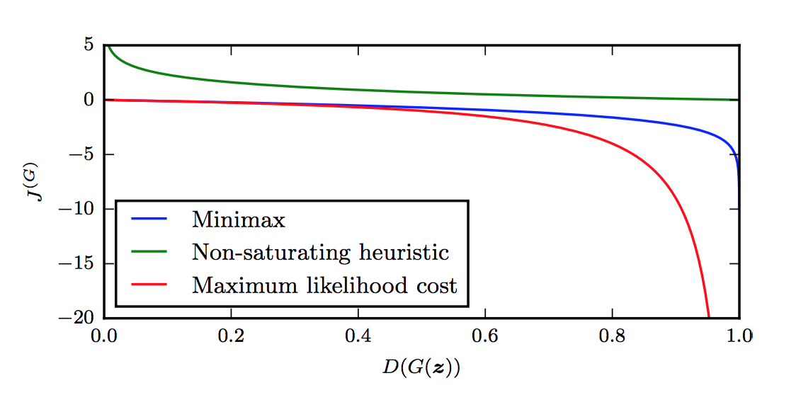
  Using Goodfellow’s notation, we have the following candidates for the generator loss function, as discussed in the tutorial. The first is the minimax version:

  \[J^{(G)} = -J^{(J)} = \frac{1}{2} \mathbb{E}_{x \sim p_{\rm data}}\Big[ \log D(x)\Big] + \frac{1}{2} \mathbb{E}_{z} \Big[\log (1-D(G(z)))\Big]\]

  The second is the heuristic, non-saturating version:

  \[J^{(G)} = -\frac{1}{2}\mathbb{E}_z\Big[\log D(G(z))\Big]\]

  Finally, the third is the maximum likelihood version:

  \[J^{(G)} = -\frac{1}{2}\mathbb{E}_z\left[e^{\sigma^{-1}(D(G(z)))}\right]\]

  What are the advantages and disadvantages of these generator loss functions? For the minimax version, it’s simple and allows for easier theoretical results, but in practice its not that useful, due to gradient saturation. As Goodfellow notes:

  In the minimax game, the discriminator minimizes a cross-entropy, but the generator maximizes the same cross-entropy. This is unfortunate for the generator, because when the discriminator successfully rejects generator samples with high confidence, the generator’s gradient vanishes.

  As suggested in Chapter 3 of Michael Nielsen’s excellent online book, the cross-entropy is a great loss function since it is designed in part to accelerate learning and avoid gradient saturation only up to when the classifier is correct (since we don’t want the gradient to move in that case!).

  I’m not sure how to clearly describe this formally. For now, I will defer to Figure 16 in Goodfellow’s tutorial (see the top of this blog post), which nicely shows the value of \(J^{(G)}\) as a function of the discriminator’s output, \(D(G(z))\). Indeed, when the discriminator is winning, we’re at the left side of the graph, since the discriminator outputs the probability of the sample being from the true data distribution.

  By the way, why is \(J^{(G)} = -J^{(J)}\) only a function of \(D(G(z))\) as suggested by the figure? What about the other term in \(J^{(J)}\)? Notice that of the two terms in the loss function, the first one is only a function of the discriminator’s parameters! The second part, which uses the \(D(G(z))\) term, depends on both \(D\) and \(G\). Hence, for the purposes of performing gradient descent with respect to the parameters of \(G\), only the second term in \(J^{(J)}\) matters; the first term is a constant that disappears after taking derivatives \(\nabla_{\theta^{(G)}}\).

  The figure makes it clear that the generator will have a hard time doing any sort of gradient update at the left portion of the graph, since the derivatives are close to zero. The problem is that the left portion of the graph represents the most common case when starting the game. The generator, after all, starts out with basically random parameters, so the discriminator can easily tell what is real and what is fake.²

  Let’s move on to the other two generator cost functions. The second one, the heuristically-motivated one, uses the idea that the generator’s gradient only depends on the second term in \(J^{(J)}\). Instead of flipping the sign of \(J^{(J)}\), they instead flip the target: changing \(\log (1-D(G(z)))\) to \(\log D(G(z))\). In other words, the “sign flipping” happens at a different part, so the generator still optimizes something “opposite” of the discriminator. From this re-formulation, it appears from the figure above that \(J^{(G)}\) now has desirable gradients in the left portion of the graph. Thus, the advantage here is that the generator gets a strong gradient signal so that it can quickly improve. The downside is that it’s not easier to analyze, but who cares?

  Finally, the maximum likelihood cost function has the advantage of being motivated based on maximum likelihood, which by itself has a lot of desirable properties. Unfortunately, the figure above shows that it has a flat slope in the left portion, though it seems to be slightly better than the minimax version since it decreases rapidly “sooner.” Though that might not be an “advantage,” since Goodfellow warns about high variance. That might be worth thinking about in more detail.

  One last note: the function \(J^{(G)}\), at least for the three cost functions here, does not depend directly on \(x\) at all! That’s interesting … and in fact, Goodfellow argues that makes GANs resistant to overfitting since it can’t copy from \(x\).

I wish more tutorials like this existed for other AI concepts. I particularly enjoyed the three exercises and the solutions within this tutorial on GANs. I have more detailed notes here in my Paper Notes GitHub repository (I should have started this repository back in 2013). I highly recommend this tutorial to anyone wanting to know more about GANs.

Update March 26, 2020: made a few clarifications.