Understanding Deep Learning Requires Rethinking Generalization: My Thoughts and Notes
The paper “Understanding Deep Learning Requires Rethinking Generalization” (arXiv link) caused quite a stir in the Deep Learning and Machine Learning research communities. It’s the rare paper that seems to have high research merit — judging from being awarded one of three Best Paper awards at ICLR 2017 — but is also readable. Hence, it got the most amount of comments of any ICLR 2017 submission on OpenReview. It has also been discussed on reddit and was recently featured on The Morning Paper blog. I was aware of the paper shortly after it was uploaded to arXiv, but never found the time to read it in detail until now.
I enjoyed reading the paper, and while I agree with many readers that some of the findings might be obvious, the paper nonetheless seems deserving of the attention it has been getting.
The authors conveniently put two of their important findings in centered italics:
Deep neural networks easily fit random labels.
and
Explicit regularization may improve generalization performance, but is neither necessary nor by itself sufficient for controlling generalization error.
I will also quote another contribution from the paper that I find interesting:
We complement our empirical observations with a theoretical construction showing that generically large neural networks can express any labeling of the training data.
(I go through the derivation later in this post.)
Going back to their first claim about deep neural networks fitting random labels, what does this mean from a generalization perspective? (Generalization is just the difference between training error and testing error.) It means that we cannot come up with a “generalization function” that can take in a neural network as input and output a generalization quality score. Here’s my intuition:
-
What we want: let’s imagine an arbitrary encoding of a neural network designed to give as much deterministic information as possible, such as the architecture and hyperparameters, and then use that encoding as input to a generalization function. We want that function to give us a number representing generalization quality, assuming that the datasets are allowed to vary. The worst generalization occurs when a fixed neural network gets excellent training error but could get either the same testing error (awesome!), or get test-set performance no better than random guessing (ugh!).
-
Reality: unfortunately, the best we can do seems to be no better than the worst case. We know of no function that can provide bounds on generalization performance across all datasets. Why? Let’s use the LeNet architecture and MNIST as an example. With the right architecture, generalization error is very small as both training and testing performance are in the high 90 percentages. With a second data set that consists of the same MNIST digits, but with the labels randomized, that same LeNet architecture can do no better than random guessing on the test set, even though the training performance is extremely good (or at least, it should be). That’s literally as bad as we can get. There’s no point in developing a function to measure generalization when we know it can only tell us that generalization will be in between zero (i.e. perfect) and the difference between zero and random guessing (i.e. the worst case)!
As they later discuss in the paper, regularization can be used to improve generalization, but will not be sufficient for developing our desired generalization criteria.
Let’s briefly take a step back and consider classical machine learning, which provides us with generalization criteria such as VC-dimension, Rademacher complexity, and uniform stability. I learned about VC-dimension during my undergraduate machine learning class, Rademacher complexity during STAT 210B this past semester, and … actually I’m not familiar with uniform stability. But intuitively … it makes sense to me that classical criteria do not apply to deep networks. To take the Rademacher complexity example: a function class which can fit to arbitrary \(\pm 1\) noise vectors presents the trivial bound of one, which is like saying: “generalization is between zero and the worst case.” Not very helpful.
The paper then proceeds to describe their testing scenario, and packs some important results in the figure reproduced below:
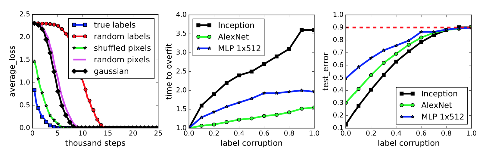
This figure represents a neural network classifying the images in the widely-benchmarked CIFAR-10 dataset. The network the authors used is a simplified version of the Inception architecture.
-
The first subplot represents five different settings of the labels and input images. To be clear on what the “gaussian” setting means, they use a Gaussian distribution to generate random pixels (!!) for every image. The mean and variance of that Gaussian are “matched to the original dataset.” In addition, the “shuffled” and “random” pixels apply a random permutation to the pixels, with the same permutation to all images for the former, and different permutations for the latter.
We immediately see that the neural network can get zero training error on all the settings, but the convergence speed varies. Intuition suggests that the dataset with the correct labels and the one with the same shuffling permutation should converge quickly, and this indeed is the case. Interestingly enough, I thought the “gaussian” setting would have the worst performance, but that prize seems to go to “random labels.”
-
The second subplot measures training error when the amount of label noise is varied; with some probability \(p\), each image independently has its labeled corrupted and replaced with a draw from the discrete uniform distribution over the classes. The results show that more corruption slows convergence, which makes sense. By the way, using a continuum of something is a common research tactic and something I should try for my own work.
-
Finally, the third subplot measures generalization error under label corruption. As these data points were all measured after convergence, this is equivalent to the test error. The results here also make a lot of sense. Test set error should be approaching 90 percent because CIFAR-10 has 10 classes (that’s why it’s called CIFAR-10!).
My major criticism of this figure is not that the results, particularly in the second and third subplots, might seem obvious but that the figure lacks error bars. Since it’s easy nowadays to program multiple calls in a bash script or something similar, I would expect at least three trials and with error bars (or “regions”) to each curve in this figure.
The next section discusses the role of regularization, which is normally applied to prevent overfitting to the training data. The classic example is with linear regression and a dataset of several points arranged in roughly a linear fashion. Do we try to fit a straight line through these points, which might have lots of training error, or do we take a high-dimensional polynomial and fit every point exactly, even if the resulting curve looks impossibly crazy? That’s what regularization helps to control. Explicit regularization in linear regression is the \(\lambda\) term in the following optimization problem:
\[\min_w \|Xw - y\|_2^2 + \lambda \|w\|_2^2\]I presented this in an earlier blog post.
To investigate the role of regularization in Deep Learning, the authors test with and without regularizers. Incidentally, the use of \(\lambda\) above is not the only type of regularization. There are also several others: data augmentation, dropout, weight decay, early stopping (implicit) and batch normalization (implicit). These are standard tools in the modern Deep Learning toolkit.
They find that, while regularization helps to improve generalization performance, it is still possible to get excellent generalization even with no regularization. They conclude:
In summary, our observations on both explicit and implicit regularizers are consistently suggesting that regularizers, when properly tuned, could help to improve the generalization performance. However, it is unlikely that the regularizers are the fundamental reason for generalization, as the networks continue to perform well after all the regularizers [are] removed.
On a side note, the regularization discussion in the paper feels out of order and the writing sounds a bit off to me. I wish they had more time to fix this, as the regularization portion of the paper contains most of my English language-related criticism.
Moving on, the next section of the paper is about finite-sample expressivity, or understanding what functions neural networks can express given a finite number of samples. The authors state that the previous literature focuses on population analysis where one can assume an arbitrary number of samples. Here, instead, they assume a fixed set of \(n\) training points \(\{x_1,\ldots,x_n\}\). This seems easier to understand anyway.
They prove a theorem that relates to the third major contribution I wrote earlier: “that generically large neural networks can express any labeling of the training data.” Before proving the theorem, let’s begin with the following lemma:
Lemma 1. For any two interleaving sequences of \(n\) real numbers
\[b_1 < x_1 < b_2 < x_2 \cdots < b_n < x_n\]the \(n \times n\) matrix \(A = [\max\{x_i - b_j, 0\}]_{ij}\) has full rank. Its smallest eigenvalue is \(\min_i (x_i - b_i)\).
Whenever I see statements like these, my first instinct is to draw out the matrix. And here it is:
\[\begin{align} A &= \begin{bmatrix} \max\{x_1-b_1, 0\} & \max\{x_1-b_2, 0\} & \cdots & \max\{x_1-b_n, 0\} \\ \max\{x_2-b_1, 0\} & \max\{x_2-b_2, 0\} & \cdots & \max\{x_2-b_n, 0\} \\ \vdots & \ddots & \ddots & \vdots \\ \max\{x_n-b_1, 0\} & \max\{x_n-b_2, 0\} & \cdots & \max\{x_n-b_n, 0\} \end{bmatrix} \\ &\;{\overset{(i)}{=}}\; \begin{bmatrix} x_1-b_1 & 0 & 0 & \cdots & 0 \\ x_2-b_1 & x_2-b_2 & 0 & \cdots & 0 \\ \vdots & \ddots & \ddots & \ddots & \vdots \\ x_{n-1}-b_1 & x_{n-1}-b_2 & \ddots & \cdots & 0 \\ x_n-b_1 & x_n-b_2 & x_n-b_3 & \cdots & x_n-b_n \end{bmatrix} \end{align}\]where (i) follows from the interleaving sequence assumption. This matrix is lower-triangular, and moreover, all the non-zero elements are positive. We know from linear algebra that lower triangular matrices
- are invertible if and only if the diagonal elements are nonzero
- have their eigenvalues taken directly from the diagonal elements
These two facts together prove Lemma 1. Next, we can prove:
Theorem 1. There exists a two-layer neural network with ReLU activations and \(2n + d\) weights that can represent any function on a sample of size \(n\) in \(d\) dimensions.
Consider the function
\[c(x) = \sum_{j=1}^n w_j \cdot \max\{a^Tx-b_j,0\}\]with \(w, b \in \mathbb{R}^n\) and \(a,x\in \mathbb{R}^d\). (There’s a typo in the paper, \(c\) is a function from \(\mathbb{R}^d\to \mathbb{R}\), not \(\mathbb{R}^n\to \mathbb{R}\)). This can certainly be represented by a depth-2 ReLU network. To be clear on the naming convention, “depth-2” does not count the input layer, so our network should only have one ReLU layer in it as the output shouldn’t have ReLUs applied to it.
Here’s how to think of the network representing \(c\). First, assume that we have a minibatch of \(n\) elements, so that \(X\) is the \(n\times d\) data matrix. The depth-2 network representing \(c\) can be expressed as:
\[c(X) = \max\left( \underbrace{\begin{bmatrix} \texttt{---} & x_1 & \texttt{---} \\ \vdots & \vdots & \vdots \\ \texttt{---} & x_n & \texttt{---} \\ \end{bmatrix}}_{n\times d} \underbrace{\begin{bmatrix} \mid & & \mid \\ a & \cdots & a \\ \mid & & \mid \end{bmatrix}}_{d \times n} - \underbrace{\begin{bmatrix} b_1 & \cdots & b_n \end{bmatrix}}_{1\times n} , \;\; \underbrace{\begin{bmatrix} 0 & \cdots & 0 \end{bmatrix}}_{1\times n} \right) \cdot \begin{bmatrix} w_1 \\ \vdots \\ w_n \end{bmatrix}\]where \(b\) and the zero-vector used in the maximum “broadcast” as necessary in Python code.
Given a fixed dataset \(S=\{z_1,\ldots,z_n\}\) of distinct inputs with labels \(y_1,\ldots,y_n\), we must be able to find settings of \(a,w,\) and \(b\) such that \(c(z_i)=y_i\) for all \(i\). You might be guessing how we’re doing this: we must reduce this to the interleaving property in Lemma 1. Due to the uniqueness of the \(z_i\), it is possible to find \(a\) to make the \(x_i=z_i^Ta\) terms satisfy the interleaving property. Then we have a full rank solution, hence \(y=Aw\) results in \(w^* = A^{-1}y\) as our final weights, where \(A\) is precisely that matrix from Lemma 1! We also see that, indeed, there are \(n+n+d\) weights in the network. This is an interesting and fun proof, and I think variants of this question would work well as a homework assignment for a Deep Learning class.
The authors conclude the paper by trying to understand generalization with linear models, in the hope that some of the intuition will transfer over to the Deep Learning setting. With linear models, given some weights \(w\) resulting from the optimization problem, what can we say about generalization just by looking at it? Curvature is one popular metric to understand the quality of the minima (which is not necessarily the same as the generalization criteria!), but the Hessian is independent of \(w\), so in fact it seems impossible to use curvature for generalization. I’m convinced this is true for the normal mean square loss, but is this still true if the loss function were, say, the cube of the \(L_2\) difference? After all, there are only two derivatives applied on \(w\), right?
The authors instead urge us to think of stochastic gradient descent instead of curvature when trying to measure quality. Assuming that \(w_0=0\), the stochastic gradient descent update consists of a series of “linear combination” updates, and hence the result is just a linear combination of linear combinations of linear combinations … (and so forth) … which at the end of the day, remains a linear combination. (I don’t think they need to assume \(w_0=0\) if we can add an extra 1 to all the data points.) Consequently, they can fit any set of labels of the data by solving a linear equation, and indeed, they get strong performance on MNIST and CIFAR-10, even without regularization.
They next try to relate this to a minimum norm interpretation, though this is not a fruitful direction because their results are worse when they try to find minimum norm solutions. On MNIST, their best solution using some “Gabor wavelet transform” (what?), is twice as better as the minimum norm solution. I’m not sure how much stock to put into this section, other than how I like their perspective of thinking of SGD as an implicit regularizer (like batch normalization) rather than an optimizer. The line between the categories is blurring.
To conclude, from my growing experience with Deep Learning, I don’t find their experimental results surprising. That’s not to say the paper was entirely predictable, but think of it this way: if I were a computer vision researcher pre-AlexNet, I would be more surprised at reading the AlexNet paper as I am today reading this paper. Ultimately, as I mentioned earlier, I enjoyed this paper, and while it was predictable (that word again…) that it couldn’t offer any solutions, perhaps it will be useful as a starting point to understanding generalization in Deep Learning.