Learning to Act by Predicting the Future
I first heard about the paper Learning to Act by Predicting the Future after one of the authors, Vladlen Koltun, came to give a highly entertaining talk as part of Berkeley’s Deep Learning seminar course (CS 294-131).
In retrospect, I’m embarrassed it took me this long to find out about the work. It’s research that feels highly insightful and should have been clear to us all along — yet somehow we never saw it until those authors presented it to us. To me, that’s an indicator of high-caliber research.
Others have agreed. Learning to Act by Predicting the Future was accepted as an oral presentation at ICLR 2017, meaning that it was one of the top 15 or so papers. You can check out the favorable reviews on OpenReview. It was also featured on Adrian Colyer’s blog. And of course, it was featured in my Deep Learning class.
So what is the research contribution of the paper? Here’s a key passage in the introduction which explains their framework:
Our approach departs from the reward-based formalization commonly used in RL. Instead of a monolithic state and a scalar reward, we consider a stream of sensory input \(\{s_t\}\) and a stream of measurements \(\{m_t\}\). The sensory stream is typically high-dimensional and may include the raw visual, auditory, and tactile input. The measurement stream has lower dimensionality and constitutes a set of data that pertain to the agent’s current state.
To be clear, at each time \(t\), we get one sensory input and one set of (scalar-valued) measurements, so our observation is \(o_t = \langle s_t, m_t \rangle\). Their running test platform in the paper is the first-person shooter Doom environment, so \(s_t\) represents images and \(m_t\) represents attributes in the game such as health and supply levels.
This is an intuitive difference between \(s_t\) and \(m_t\). There are, however, two important algorithmic differences:
-
Given actions taken by the agent, they attempt to predict \(m_t\), hence “predicting the future”. It’s very hard to predict full-blown images, but predicting (much-smaller) measurements shouldn’t be nearly as challenging.
-
The measurement vector \(m_t\) is used to shape the agent’s goals. They assume the agent wants to maximize
\[u(f;g) = g^\top f\]where
\[f = \langle m_{t+\tau_1}-m_t, \ldots, m_{t+\tau_n}-m_t\rangle\]Thus, the goal is to maximize this inner product of the future measurements and a parameter vector \(g\) weighing the relative importance of each terms. Note that this instantly generalizes the case with a scalar reward signal in MDPs: we’d set the elements of \(g\) such that they are \(\gamma^0, \gamma^1, \gamma^2, \ldots\), i.e. corresponding to discounted rewards. (I’m assuming that \(m_t\) is a scalar here, but this generalizes to the vector case with \(f\) a matrix, as we could flatten \(f\) and \(g\).)
In order to predict \(m_t\), they have to train a function to do so, which they parameterize with (you guessed it) deep neural networks. They define the function \(F\) as the predictor, with
\[p_t^a = F(o_t, a_t, g ; \theta)\]Thus, given the observation, action, and goal vector parameter, we can predict the resulting measurements, so that during test-time applications, \(p_t^a\) is “plugged in” for \(f\) and the action which maximizes \(u\) is chosen. To make this work mathematically, of course, \(f,g,\) and \(p_t^a\) must all have the same dimension. And to be clear, even though the reward (as they define it) is a function of \(g\), we are not “training” the \(g\) parameters but the parameters for \(F\).
The parameters of \(F\), incidentally, are trained in an unsupervised manner, or using “self-supervision” since the labels can be generated automatically by having the agent wander around in the world and then repeatedly computing the value of the function output at each of those time steps. Then, after some time has passed, we simply minimize the \(L_2\) loss. Nice, no humans needed for labeling! When I was reading this, I was reminded of the Q-learning update, since the update rule automatically assumes that the “target” is the usual “reward plus discounted max Q-value” thingy, without human intervention. To further the connection with Q-learning, they use an experience memory in the same way as the DQN algorithm used experience replay (see my earlier blog post about DQN). Another concept that came to mind was Sergey Levine’s excellent paper on learning hand-eye coordination, where he and his collaborators were able to automatically generate labels. I need to figure out how to do stuff like this more often.
Anyway, given that \(F\) takes in three inputs, one would intuitively expect that it has three separate input networks and concatenates them at some point. Indeed, that’s what they do in their network, shown below.
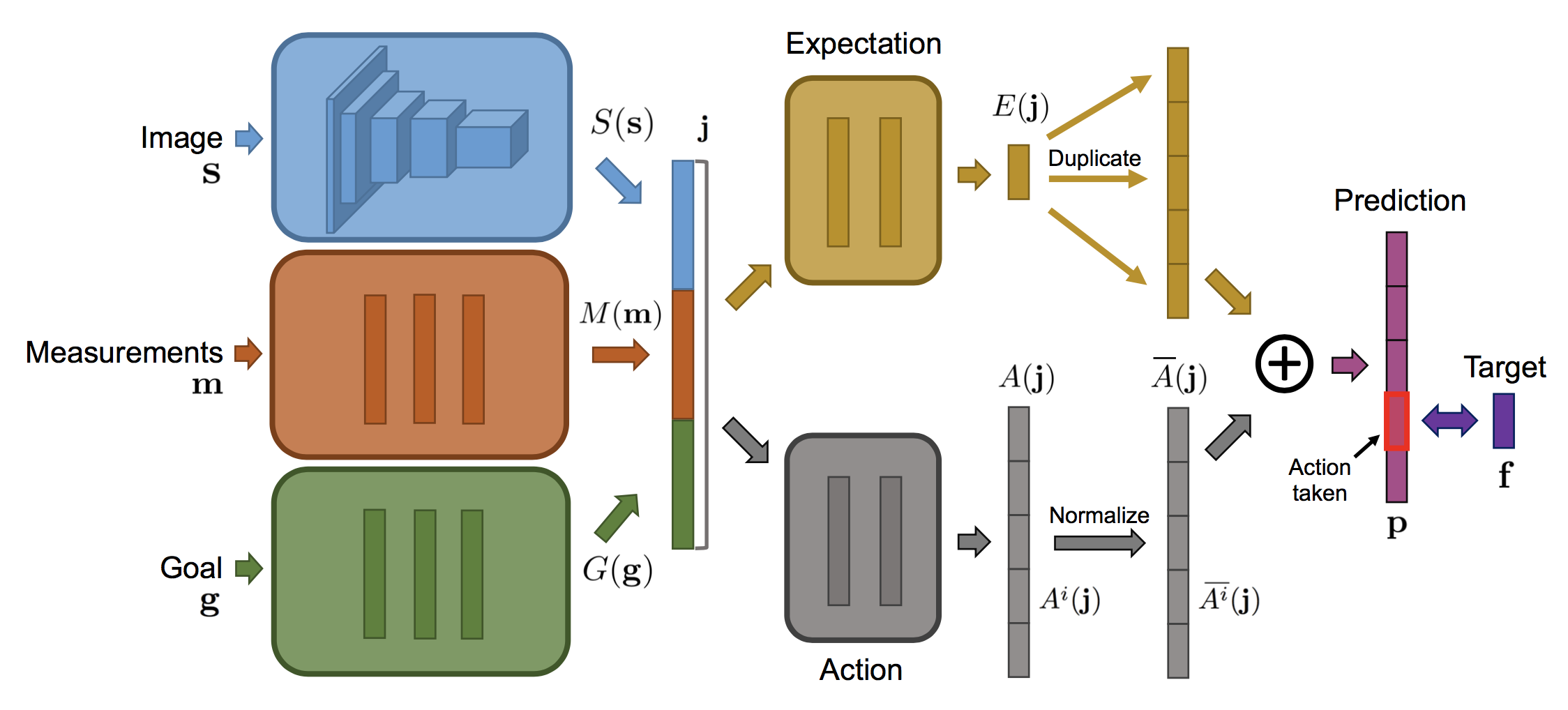
After concatenation, the network follows the paradigm of the Dueling DQN architecture by having separate expectation and value (“action”) streams. It might not be clear why this is useful, so if you’re puzzled, I recommend reading the Dueling DQN paper for justification (I need to re-read that as well).
They benchmark their paradigm (called DFP for “Direct Future Prediction”) on Doom with four scenarios of increasing difficulty. The baselines are the well-known DQN and A3C algorithms, along with a relatively obscure “DSR” algorithm (but which used the Doom platform, facilitating comparisons). I’m not sure why they used DQN instead of, say, Double DQN or prioritized variants since those are assumed to be strictly better, but at least they test using A3C which as far as I can tell is on par with the best DQN variants. It’s too bad that OpenAI baselines wasn’t around in time for the authors to use it for this paper.
They say that
We set the temporal offsets \(\tau_1, \ldots, \tau_n\) of predicted future measurements to 1, 2, 4, 8, 16, and 32 steps in all experiments. Only the latest three time steps contribute to the objective function, with coefficients \((0.5, 0.5, 1)\).
I think they say this to mean that their goal vector \(g\) contains only three nonzero components, corresponding to \(\tau_{n-2}, \tau_{n-1}\) and \(\tau_n\). But then I’m confused: why do they need to have all the other \(\tau_i\) for \(1 \le i \le n-3\)? What’s also confusing is that for the two complicated environments with ammo, health, and frags, their training is set to maximize a linear combination of those three, with coefficients \((0.5, 0.5, 1.0)\). The same vector is repeated here!
I wish they had expanded upon their discussion since this is new stuff from their paper. Why did they choose this and that value? What is the intuition? I know it’s easy to ask this from a reading/reviewing perspective, but that’s only because the concept is new; for example, they do not need to justify why they chose the dueling-style architecture because they can refer to the Dueling DQN paper.
Regarding experiments, I don’t have much intuition on the vizDoom environments, as I have never used those, but their results look impressive on the two harder scenarios, which also provide more measurements (three instead of one). Their method out-performs sophisticated baselines in various settings, including those from the Visual Doom AI competition in September 2016.
At the end of the experimental section, after a few ablation studies (heh, my favorite!) they convincingly claim that
This supports the intuition that a dense flow of multivariate measurements is a better training signal than a scalar reward.
In my words: dense signals are better than sparse signals. In some cases, sparsity is desirable (e.g. in attention models, we want sparsity to focus on a few important components) but for rewards in reinforcement learning, we definitely need dense signals. Note that getting such signals wouldn’t be possible if the authors kept clinging to the usual MDP formulation. Indeed, Koltun made it a point in his talk to emphasize how he disagreed with the constraints imposed on us by the MDP formulation, with the usual “set of states, actions, rewards […]”. This is one of the things I wish I was better at: identifying certain gaps in assumptions that everyone makes, and trying to figure out where we can improve them.
That’s all I have to say for this paper now. For more details, I would check the paper website. Have fun!