Basics of Bayesian Neural Networks

In this post, I try and learn as much about Bayesian Neural Networks (BNNs) as I can. I borrow the perspective of Radford Neal: BNNs are updated in two steps. The first step samples the hyperparameters, which are typically the regularizer terms set on a per-layer basis. The second step performs Hamiltonian Monte Carlo over the data, or through a series of minibatches plus sophisticated “friction” techniques, if using Stochastic Gradient Hamiltonian Monte Carlo. These update the actual weights we use for the neural networks; the hyperparameters are sampled mainly to invoke a “fully Bayesian” hierarchical model.

The above is different from the paradigm of using Bayesian Neural Networks with a technique known as variational inference. I will not be discussing that.

To make things concrete, in this blog post I will assume we have the following neural network which:

• is fully connected.
• takes MNIST data as input (784 dimensions for each data point), has a hidden layer of 100 units, and outputs a 10-dimensional vector from a softmax.
• uses the sigmoid activation for the hidden layer.
• uses a regularizer hyperparameter for each of the two sets of weight matrices, along with two for the biases.

We can write the network’s mathematical meaning using \(A \in \mathbb{R}^{10 \times 100}\) and \(B \in \mathbb{R}^{784 \times 100}\) as the weight matrices, along with \(a \in \mathbb{R}^{10}\) and \(b \in \mathbb{R}^{100}\) as the bias vectors. Using this, the network output can be expressed as:

where \(y \in \{0,1,\ldots,9\}\) indicates the class label and \(A_i\) is the \(i\)th column of \(A\). (The entire output would just be the vector of \(\langle P(y=0| x), \ldots, P(y=9| x)\rangle\) values.) I write \((x,y)\) without subscripts, but in general we should write \(\mathcal{D} = \{(x^{(k)},y^{(k)})\}_{k=1}^N\) to represent the entire dataset.

We need to incorporate Bayesian assumptions somehow, so first we assume that all these weights have Gaussian priors with zero mean and covariance matrix \(\Sigma = \sigma_A^2 I\) set to some multiple of the identity. Intuitively, this seems to be a reasonable prior, as we’d generally like our weights to be small and roughly symmetrical about zero. For example, with the weights for \(A\), we

where we set \(\lambda_A\) to be the inverse variance, also known as the precision term. Similarly, we have \(P(B) \propto \exp\left(-\frac{\lambda_B}{2}\|B\|_2^2\right)\), \(P(a) \propto \exp\left(-\frac{\lambda_a}{2}\|a\|_2^2\right)\), and \(P(b) \propto \exp\left(-\frac{\lambda_b}{2}\|b\|_2^2\right)\). Notice that I am now flattening the matrices \(A\) and \(B\) so that they are vectors. This makes the notation a bit easier, and it means that when I write \(\|A\|_2\), I mean the \(L_2\) norm, not the spectral norm on matrices (a.k.a., the largest singular value). I will use the flattened notation for the remainder of this blog post.

The precision terms are hyperparameters which we also endow with their own (IID) priors:¹

Letting \(\Theta\) denote our eight major parameters (including the hyperparameters), the posterior distribution which we want to sample from based on dataset \(\mathcal{D}\) is

where we follow the usual assumption of conditional independence among the data; think of drawing data points from the true “data distribution” to form our training data.

BNNs use Bayesian methods to figure out a good set of parameters \(\Theta\) for some task, which here is based on digit classification accuracy. I will now go over how the hyperparameter updates work, followed by the parameter updates.

The Hyperparameter Updates

This step samples the following:

There is no dependence on the dataset \(\mathcal{D}\) as the hyperparameters are sampled based on “data” which consists of the parameter values at the lower level. Also, since we assumed an IID prior for the precision terms, and because the values of the parameters are viewed as independent as well (I admit this probably isn’t the best way of describing it but it feels intuitive) we have:

We can literally sample the four precision terms sequentially due to their independence assumptions. For simplicity, let us assume we are sampling only \(\lambda_A\) so that the rest of the computation is straightforward. The math turns out to be:

and indeed, we have conjugacy: sampling the hyperparameters can be done simply by sampling from a Gamma distribution with these updated parameters based on the previous values of \(\alpha\) and \(\beta\). For intuition on what these parameters mean, if we have \(X \sim \Gamma(\alpha, \beta)\), then \(\mathbb{E}[X] = \alpha / \beta\).

The Parameter Updates

This step samples the following:

where \(\Lambda = \{\lambda_A,\lambda_B, \lambda_a, \lambda_b\}\) to simplify the notation if we depend on all the hyperparameters. There is dependence on \(\Lambda\) here as those values determine the spread of the Gaussian distributions. Also, notice the dependence on the data here, unlike the previous case.

Using Bayes’ Rule as we did earlier (with that condensed \(\Theta\) notation) we get:

How do we sample from this distribution? We use Hamiltonian Monte Carlo (HMC).

The Hamiltonian, Potential Energy, and Kinetic Energy

Briefly: HMC uses what is known as a Hamiltonian Function \(H(\Theta,p)\) where \(\Theta\) are the parameters and \(p\) refers to auxiliary momentum variables.² In Bayesian statistics, current practice is to split the Hamiltonian into two functions: \(H(\Theta,p) = U(\Theta) + K(p)\) known as the potential energy and kinetic energy, respectively. HMC is designed to sample from the distribution defined as follows:

where \(Z>0\) is a normalizing constant and \(T>0\) is some temperature, typically used to “flatten” or “diffuse” the target distribution (which here is \(\propto \exp\left(-\frac{H(\Theta,p)}{T}\right)\)) to make optimization easier. For the rest of this post, I include \(T\) for clarity but I keep it separate from \(H, U,\) and \(K\).

In Bayesian statistics, the Potential Energy is \(U(\Theta) = -\log(P(\Theta) \cdot P(\mathcal{D} | \Theta))\) because if we plug that in, we get

which is exactly what we want for the position variables, assuming that the momentum is independent so that \(P(\Theta,p)=P(\Theta)P(p)\), which is standard practice. To be clear: (a) we’re only interested in sampling from the distribution for \(\Theta\), not the momentum’s distribution, so (b) to get our desired samples of \(\Theta\) from the posterior, we generate samples \((\Theta^{(i)},p^{(i)})\) that include the momentum variables, and then we drop the latter after we’re done.

Regarding the Kinetic Energy, current practice is to set it to be a quadratic potential with mass matrix \(M = \sigma^2 I\) a multiple of the identity:

To be clear, we need to sample from the target distribution as specified by \(\exp\left(-\frac{H(\Theta,p)}{T}\right)\), which means we must technically sample from the distributions defined as:

Here, \(U\) and \(K\) are energy functions, but they are not the same as the actual distribution we are sampling from. For example, with the kinetic energy, the actual distribution we sample from is proportional to

i.e., a zero-mean Gaussian with covariance \(T\sigma^2I\). We sequentially sample for each because they are independent by assumption.

Running Hamiltonian Monte Carlo

Running HMC in computer simulation requires a Metropolis test³ each iteration (i.e., each sample in our MCMC chain) to correct for discretization error. This requires computing the follow ratio \(r\):

where \(\Theta'\) and \(p'\) refer to the proposed position and momentum variables, respectively. Computing the kinetic energy is typically a matter of adding squared \(L_2\) norms, so that part is easy. But what about \(U\)? To compute this difference for our proposed Bayesian Neural Network, we see that

where \(C\) represents a constant independent of the parameter \(\Theta\). The reason why I ignore this is twofold.

• First, when computing the Metropolis ratio, that \(C\) will be the same for both \(U(\Theta)\) and \(U(\Theta')\) so we can ignore it.

• Second, we also need to use \(U\) when we sample with HMC, and this means taking the gradient \(\nabla_\Theta U(\Theta)\) which will kill \(C\). (The Metropolis test is only to determine whether we accept or reject a proposal, but we need some way of actually getting that proposal).

To elaborate on the second point, sampling using “Hamiltonian Dynamics” requires the momentum update:

where \(\epsilon\) is a (leapfrog) step size parameter which we divide by two as required from the leapfrog method.

You can immediately see from this that \(p\) must have the same dimensions as \(\Theta\). I think of \(p\) as concatenating flattened \(A,B,a,b\) weights, so it’s one giant vector. The gradient updates can be specified weight-by-weight, which will change the corresponding “slices” of the vector \(p\). For instance, with \(A\) and abusing notation by re-using \(p\), we have:

The \(\lambda_A A\) term serves as a weight decay regularizer, and the sum over the gradient of probabilities can be computed via backpropagation through the neural network.

• Remark 1: hopefully my above explanation clarifies why imposing a Gaussian prior on the weights is equivalent to \(L_2\) regularization.

• Remark 2: consider using TensorFlow to get the gradients corresponding to the log probabilities. In particular, TensorFlow can return gradients using tf.gradients.

One thing I should point out: here, we can view \(- \log P(\mathcal{D} | \Theta; \Lambda)\) as a “cost function” that we’re trying to minimize. This is equivalent to minimizing the cross entropy loss between what our the neural network predicts, and the distribution that consists of one-hot vectors of the training labels.⁴ That’s precisely the loss function I’d use if I were formulating the classification problem and solving it with stochastic gradient descent instead of HMC. The implication is that it’s OK to try and maximize the \(\log P(y^{(k)} | x^{(k)}, \Theta ; \Lambda)\) value that we see above, which is what happens when we perform gradient ascent on it; intuitively, the resulting weights will assign higher probability to the correct class.

After the momentum updates, the position variables are updated using a similar gradient-based step:

so that, intuitively, \(\Theta\) is also updated in roughly the same direction of the gradient. That’s how HMC works and uses gradient information.

Practical Considerations

Averaging Predictions

Using Bayesian Neural Networks in practice often requires sampling a set of neural network weights many times and then computing the mean and standard deviation of the predictions.

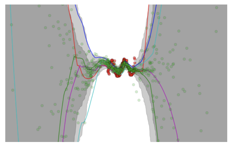
A figure copied from the VIME paper (NIPS 2016) showing Bayesian Neural Network predictions and uncertainty levels.

For instance, in the figure above (taken from the VIME paper) the authors construct a regression task, where the network takes in a scalar-valued⁵ input \(x \in \mathbb{R}\) and outputs a prediction \(y \in \mathbb{R}\). The red dots are the targets, while the green dots are the predictions. It’s clear that the red dots are clustered near the center of the figure, so logically, our Bayesian Neural Networks should be very confident in their predictions in those areas, and less confident outside the training data’s dominant regime. Indeed, the shaded areas confirm this, as they represent the output mean plus/minus one and two standard deviations (I think the second standard deviation is too far to see for the extremes in this figure) based on different neural network weight parameters.

These types of figures are typically shown when people talk about Bayesian Neural Networks, such as in Yarin Gal’s excellent tutorial.

Code Implementation

I am working on implementing Bayesian Neural Networks in my MCMC repository, which is a TensorFlow implementation based on Tianqi Chen’s earlier pure numpy code. The code is a bit disorganized and not quite ready for consumption by the public, but I think I’m getting something going with this code.