On the Momentum Sign Flipping for Hamiltonian Monte Carlo
For a long time, I wanted to write a nice, long, friendly blog post on Hamiltonian Monte Carlo that I could come back to for more intuition and understanding as needed.
Fortunately, there’s no need for me to invest a ginormous amount of time I don’t have for that, because physicists/statistician Michael Betancourt has written a fantastic introduction to Hamiltonian Monte Carlo, called A Conceptual Introduction to Hamiltonian Monte Carlo. You can find the preprint here on arXiv. Don’t be deterred by the length; it’s a fast read compared to other academic papers, and certainly a much more intuitive read than Radford Neal’s 2011 review chapter, which I already thought couldn’t be surpassed in terms of a quality introduction to HMC. Indeed, even prominent statisticians such as COPSS Presidents’ Award winner Andrew Gelman have praised the writeup, and someone like him obviously doesn’t need it.
I have extensively read Radford Neal’s writeup, to the point where I was able to reproduce almost all his figures in my MCMC and Dynamics code repository on GitHub. There was, however, one question I had about HMC that I didn’t feel was elaborated upon enough:
Why is it necessary to flip the sign of the momentum to induce a symmetric proposal?
Fortunately, Betancourt’s writeup comes to the rescue! Thus, in this post, I’d like to go through the details on why it is necessary to flip the sign of the momentum term in HMC.
Let \(\mathbb{Q}(q' \mid q)\) be the density function defining the current proposal method, whatever that may be. With a Gaussian proposal, we have symmetry in that \(\mathbb{Q}(q'\mid q) = \mathbb{Q}(q\mid q')\). The same is true with Hamiltonian Monte Carlo … if we handle the momentum term correctly.
Borrowing Betancourt’s notation (from Section 5.2), we’ll assume that, starting from state \((q_0,p_0)\), we integrate the dynamics for \(L\) steps to land at \((q_L,p_L)\), upon which we use that as our proposal:
\[\mathbb{Q}(q',p' \mid q_0,p_0) = \delta(q'-q_L) \delta(p'-p_L)\]where \(\delta: \mathbb{R} \to \{0,1\}\) is the Dirac delta function, and the difference \(q'-q_L\) is assumed to be real-valued; if \(q\) and \(p\) are vectors, these would need to be done component-wise and then summed up, but the same basic idea holds. Furthermore, \(q'\) and \(p'\) are “placeholder” random variables, kind of like how we often use \(X\) when writing \(\mathbb{P}[X=x]\) in introductory probability courses; \(X\) is the placeholder and \(x\) is the actual quantity.
Reading the definition straight from the Dirac delta functions, we see that our proposal density is one exactly at state \((q',p')=(q_L,p_L)\), and zero everywhere else. This makes sense because Hamiltonian dynamics are deterministic after re-sampling the momentum variables (but it’s understood that \(p_0\) represents those states after the re-sampling, not before).
The problem with this is that the proposal becomes “ill-posed”. Betancourt remarks that:
\[\frac{\mathbb{Q}(q_L,p_L \mid q_0,p_0)}{\mathbb{Q}(q_0,p_0 \mid q_L,p_L)} = \frac{1}{0}\]however, I believe that’s a typo and that the numerator and denominator should be flipped, so that the numerator contains the density of the starting state given the proposal.
Regardless, to me it doesn’t make sense to have proposal probabilities or densities with these Dirac delta functions that result in zero everywhere (that means we’d always reject samples). The following figure (from Betancourt) visually depicts the problem:
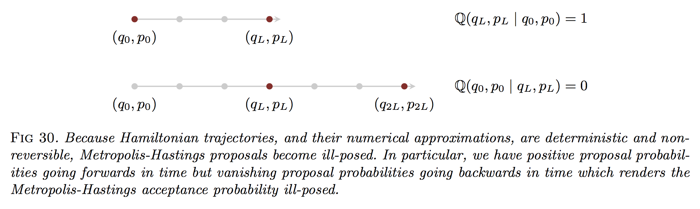
Because these position and momentum variables are continuous-valued, the probability of actually landing back in the starting state has measure zero.
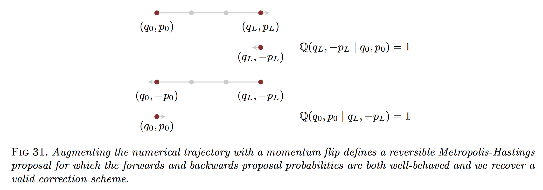
Suppose, however, that after we integrate for \(L\) steps, we flip the sign of the momentum term. Then we have
\[\mathbb{Q}(q',p' \mid q_0,p_0) = \delta(q'-q_L) \delta(p'+p_L)\]so that only \((q',p')=(q_L,-p_L)\) results in a probability mass of one. See the following figure for this revision:
The key observation now, of course, is that
\[\mathbb{Q}(q_0,p_0 \mid q_L,-p_L) = 1\]Why is this true? The dynamics are time-reversible, and if we set our potential energy to be the usual \(K(p) = \frac{p^Tp}{2}\), then flipping the momentum term and going through the leapfrog means the sampler encounters the same exact steps, only in reverse.
To make this concrete, I like to explicitly go through the math of one leapfrog step. It requires some care with notation, but I find it’s worth it. I’ll write \((q_k^{(1)},p_k^{(1)})\) as the \(k\)-th element encountered during the forward trajectory. For the reverse, I use \((q_k^{(2)},p_k^{(2)})\) so that the superscript is now two instead of one. Furthermore, due to the leapfrog step taking half-steps for momentums, I use \(k=0.5\) for this purpose.
Here’s the forward trajectory, starting from \((q_0^{(1)},p_0^{(1)})\):
\[\begin{align} p_{0.5}^{(1)} &= p_0^{(1)} - \frac{\epsilon}{2}\nabla U(q_0^{(1)}) \\ q_{1}^{(1)} &= q_0^{(1)} + \epsilon p_{0.5}^{(1)} \\ p_{1}^{(1)} &= p_{0.5}^{(1)} - \frac{\epsilon}{2}\nabla U(q_1^{(1)}) \end{align}\]and the last step negates the momentum, so that the final state is \((q_1^{(1)}, -p_1^{(1)})\).
Here’s the reverse trajectory, starting from \((q_0^{(2)},p_0^{(2)})\):
\[\begin{align} p_{0.5}^{(2)} &= p_0^{(2)} - \frac{\epsilon}{2}\nabla U(q_0^{(2)}) \\ q_{1}^{(2)} &= q_0^{(2)} + \epsilon p_{0.5}^{(2)} \\ p_{1}^{(2)} &= p_{0.5}^{(2)} - \frac{\epsilon}{2}\nabla U(q_1^{(2)}) \end{align}\]with our final state as \((q_1^{(2)}, -p_1^{(2)})\). Above, the only difference between the reverse and the forward trajectories is the change in superscripts. But when we do the math for the reverse trajectory while plugging in the values from the forward trajectory, we get:
\[\begin{align} p_{0.5}^{(2)} &= p_0^{(2)} - \frac{\epsilon}{2}\nabla U(q_0^{(2)}) \\ &= -p_1^{(1)} - \frac{\epsilon}{2}\nabla U(q_1^{(1)}) \\ &= -\left(p_{0.5}^{(1)} - \frac{\epsilon}{2}\nabla U(q_1^{(1)})\right) - \frac{\epsilon}{2}\nabla U(q_1^{(1)}) \\ &= -p_{0.5}^{(1)} \end{align}\]Gee, this is exactly the negative of the half-step we were at in the first iteration! Similarly, for the position update, we have:
\[\begin{align} q_{1}^{(2)} &= q_0^{(2)} + \epsilon p_{0.5}^{(2)} \\ &= q_1^{(1)} - \epsilon p_{0.5}^{(1)} \\ &= q_0^{(1)} + \epsilon p_{0.5}^{(1)}- \epsilon p_{0.5}^{(1)} \\ &= q_{0}^{(1)} \end{align}\]The leapfrog has brought the position back to the starting point. For the final half-step momentum update, we have:
\[\begin{align} p_{1}^{(2)} &= p_{0.5}^{(2)} - \frac{\epsilon}{2}\nabla U(q_1^{(2)}) \\ &= -p_{0.5}^{(1)} - \frac{\epsilon}{2}\nabla U(q_0^{(1)}) \\ &= -\left(p_{0}^{(1)} - \frac{\epsilon}{2}\nabla U(q_0^{(1)})\right) - \frac{\epsilon}{2}\nabla U(q_0^{(1)}) \\ &= -p_{0}^{(1)} \end{align}\]and we see that our reverse trajectory landed us back in \((q_0^{(1)},-p_0^{(1)})\), and flipping the momentum gets us to the same exact starting state.
Thus, using this type of proposal means the proposal densities cancel out, result in a Metropolis test, not a Metropolis-Hastings test.
I should also add one other point: we do not consider the momentum resampling as being part of the proposal, as resampling the momentum can be considered as maintaining the canonical distribution, so it’s something that we can “always” decide to invoke if we want (hopefully that’s not too bad of a hand-wavy explanation).
Hopefully the above discussion clarifies why flipping the sign of the momentum is necessary, at least in theory. In practice, we don’t do it since for the usual Gaussian kinetic energies, \(K(p) = K(-p)\) so their energy levels are the same, and because the momentum variables are traditionally entirely resampled after the acceptance test.