The Special Exponential Group

Over the last few weeks, I have been devouring Murray, Li, and Sastry’s A Mathematical Introduction to Robotic Manipulation. It’s freely available online and, despite the 1994 publication date, is still relevant for robotic manipulation as it’s used in EE206 at Berkeley.

(The main novelty today, from my perspective, is the use of Deep Learning to automate out analytic models under certain conditions, but I still think it’s valuable for me to know classical robotics concepts.)

In this post, I discuss the Special Exponential group, denoted as \(SE(3)\). We can define it as follows:

\[SE(3) := \{(p,R) \mid p \in \mathbb{R}^3, R \in SO(3) \}\]

where \(p\) is a position vector, and \(R\) is a matrix in the special orthogonal group \(SO(3)\):

\[SO(3) := \{R \mid R \in \mathbb{R}^{3\times 3}, R^TR=I_{3}, {\rm det}(R)=+1\}\]

This is the same as saying that \(R\) is a rotation matrix.

Side comment: the reason for “\((3)\)” as the input is that \(SE\) and \(SO\) can be generalized to an arbitrary amount of dimensions. However, I’m only concerned about robotic manipulation in \(\mathbb{R}^3\).

The above suggests the obvious question:

For what purpose do we utilize \(SE(3)\)?

We use \(SE(3)\) to encode rigid body motions (RBMs) in robotic manipulation, which preserve distance between points and angles between vectors. RBMs consist of a rotation and a translation. To visualize RBMs, look at the left of the figure below. There are two coordinate frames: frame \(A\), which is “inertial” (I think of this as the “default” frame), and frame \(B\), attached to the base of the curvy object drawn there.

Vector \(p_{ab} \in \mathbb{R}^3\) shows the 3-D position of the origin of \(B\) with respect to \(A\). This ordering from \(B\) to \(A\) and not vice versa is important, and it’s important to know these well for robotic manipulation, which in advanced contexts relies on multiple, consecutive coordinate frames attached to links in a robot arm. For rotation matrices, we’ll keep the ordering of subscripts the same and write \(R_{ab}\) to indicate that it transforms 3-D points from frame \(B\) to frame \(A\).

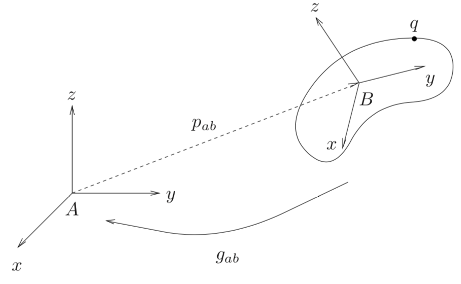
Left: visualization of two coordinate frames, one inertial and one attached to the base of an object. Right: again, two coordinate frames visualized, this time in the context of rotating about an axis.

Now consider the point \(q\) on the object. We can express its coordinates as \(q_a\) or \(q_b\), depending on which frame of \(A\) or \(B\) is our reference. Suppose we have \(q_b\). A rigid body motion can be conducted as follows:

and we’ll collect as \(g_{ab} = (p_{ab},R_{ab})\) all the information needed to specify an RBM, transforming coordinates from \(B\) to \(A\). This is an element of \(SE(3)\). Indeed, any such RBM must be an element of \(SE(3)\), which defines what’s known as a configuration space of RBMs. Configuration spaces are defined in page 25 of Murray et al:

More generally, we shall call a set \(Q\) a configuration space for a system if every element \(x\in Q\) corresponds to a valid configuration of the system and each configuration of the system can be identified with a unique element of \(Q\).

I should also provide some intuition to make it clear what happens when we “transform coordinates.” One way is as follows. If we view \(p_{ab}\) as jetting out in the positive \(x\), \(y\), and \(z\) directions of frame \(A\), and the same for \(q_b\) w.r.t. frame \(B\), then the components of \(q_a\) are element-wise larger than in \(q_b\). This is why we add when doing RBMs with translations, since the vector \(p_{ab}\) will increase the values. (Drawing a picture really helps.)

Keeping \(p_{ab}\) and \(R_{ab}\) separate can result in some cumbersome math when a bunch of rotations and translations are combined. Thus, it’s common to use homogeneous coordinates. A full discussion is beyond the scope of this blog post, but for us, the important point is that if \((p,R) \in SE(3)\), then the equivalent homogeneous representation is

where the “0” above is a row vector of three zeros. This enables us to perform one matrix-vector multiply for a 3-D point which is expanded with a fourth coordinate with a “1” in it. Thus, the origin point is \(o = (0,0,0,1)^T\), and for vectors — defined as the difference between two points — the fourth component is zero.

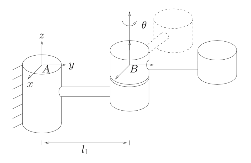
Let’s do an example. Consider the second image in the figure above, showing rotation about an axis \(\theta\). Given a fixed, “real-life”, physical point, let’s show how to encode a rigid body transformation which can transform a coordinate representation of that point from frames \(B\) to \(A\).

• Translation. Inertial frame \(A\) and frame \(B\) differ only by \(l_1\) in the y-direction, with \(p_{ab} = (0,l_1,0)^T\) representing the origin of frame \(B\) with respect to frame \(A\).

• Rotation. The rotation about \(\theta\) coincides with the \(z\) axis. Hence, we use the well-known formula for the \(z\)-axis rotation matrix:

  \[R_z(\theta) = \begin{bmatrix} \cos \theta & - \sin \theta & 0 \\ \sin \theta & \cos \theta & 0 \\ 0 & 0 & 1 \\ \end{bmatrix}\]

  While the precise positioning of the sines and cosines might not be immediately apparent, it should be clear why the last row looks like that, since a rotation about the \(z\) axis leaves the \(z\) component of the 3-D vector unchanged. You can also easily check that \(R^TR=I_3\).

  The matrix above is \(R_{ab}\), the orientation of the origin of frame \(B\) w.r.t. frame \(A\).

These two form our specification in \(SE(3)\). Combining these by using the homogeneous representation for compactness, our RBM from \(B\) to \(A\) is:

where \(\vec{a}\) and \(\vec{b}\) represent, in homogeneous coordinates, the same physical point but with respect to frames \(A\) and \(B\), respectively.