Algorithmic and Human Teaching of Sequential Decision Tasks
I spent much of the last few months preparing for the UC Berkeley EECS PhD qualifying exams, as you might have been able to tell by the style of my recent blogging (mostly paper notes) and my lack of blogging for the last few weeks. The good news is that I passed the qualifying exam. Like I did for my prelims, I wrote a “transcript” of the event. I will make it public in a future date. In this post, I discuss an interesting paper that I skimmed for my quals but didn’t have time to read in detail until after the fact: Algorithmic and Human Teaching of Sequential Decision Tasks, a 2012 AAAI paper by Maya Cakmak and Manuel Lopes.
This paper is interesting because it offers a different perspective on how to do imitation learning. Normally, in imitation learning, there is a fixed set of expert demonstrations \(D_{\rm expert} = \{\tau_1, \ldots, \tau_K \}\) where each demonstration \(\tau_i = (s_0,a_0,s_1\ldots,a_{N-1},s_N)\) is a sequence of states and actions. Then, a learner has to run some algorithm (classically, either behavior cloning or inverse reinforcement learning) to train a policy \(\pi\) that, when executed in the same environment, is as good as the expert.
In many cases, however, it makes sense that the teacher can select the most informative demonstrations for the student to learn a task. This paper thus falls under the realm of Active Teaching. This is not to be confused with Active Learning, as they clarify here:
A closely related area for the work presented in this paper is Active Learning (AL) (Angluin 1988; Settles 2010). The goal of AL, like in AT, is to reduce the number of demonstrations needed to train an agent. AL gives the learner control of what examples it is going to learn from, thereby steering the teacher’s input towards useful examples. In many cases, a teacher that chooses examples optimally will teach a concept significantly faster than an active learner choosing its own examples (Goldman and Kearns 1995).
This paper sets up the student to internally run inverse reinforcement learning (IRL), and follows prior work in assuming that the value function can be written as:
\[\begin{align*} V^{\pi}(s) \;&{\overset{(i)}=}\; \mathbb{E}_{\pi, s}\left[ \sum_{t=0}^\infty \gamma^t R(s_t)\right] \\ &{\overset{(ii)}=}\; \mathbb{E}_{\pi, s}\left[ \sum_{t=0}^\infty \gamma^t \sum_{i=1}^k w_i f_i(s_t) \right] \\ &{\overset{(iii)}=}\; \sum_{i=1}^k w_i \cdot \mathbb{E}_{\pi, s}\left[ \sum_{t=0}^\infty \gamma^t f_i(s_t)\right] \\ &{\overset{(iv)}=}\; \bar{w}^T \bar{\mu}_{\pi,s} \end{align*}\]where in (i) I applied the definition of a value function when following policy \(\pi\) (for notational simplicity, when I write a state under the expectation, like \(\mathbb{E}_s\), that means the expectation assumes we start at state \(s\)), in (ii) I substituted the reward function by assuming it is a linear combination of \(k\) features, in (iii) I re-arranged, and finally in (iv) I simplified in vector form using new notation.
We can augment the \(\bar{\mu}\) notation to also have the initial action that was chosen, as in \(s_a\). Then, using the fact that the IRL agent assumes that: “if the teacher chooses action \(a\) in state \(s\), then \(a\) must be at least as good as all the other available actions in \(s\)”, we have the following set of constraints from the demonstration data \(D\) consisting of all trajectories:
\[\forall (s,a) \in D, \forall b, \quad \bar{w}^T(\bar{\mu}_{\pi,s_a}-\bar{\mu}_{\pi,s_b}) \ge 0\]The paper’s main technical contribution is as follows. They argue that the above set of (half-space) constraints results in a subspace \(c(D)\) that contains the true weight vector, which is equivalent to obtaining the true reward function assuming we know the features. The weights are assumed to be bounded into some hypercube, \(-M_w < \bar{w} < M_w\). By sampling \(N\) different weight vectors \(\bar{w}_i\) within that hypercube, they can check the percentage of sampled weights that lie within that true subspace with this (indirect) metric:
\[G(D) = -\frac{1}{N}\sum_{i=1}^N \mathbb{1}\{\bar{w}_i \in c(D)\}\]Mathematically their problem is to find the set of demonstrations \(D\) that maximizes \(G(D)\), because if that value is larger, then the sampled weights are more likely to satisfy all the constraints, meaning that it has the property of representing the true reward function.
Note carefully: we’re allowed to change \(D\), the demonstration set, but we can’t change the way the weights are sampled: they have to be sampled from a fixed hypercube.
Their algorithm is simple: do a greedy approximation. First, select a starting state. Then, select the demonstration \(\tau_j\) that increases the current \(G( \{D \cup \tau_j \} )\) value the most. Repeat until \(G(D)\) is high enough.
For experiments, the paper relies on two sets of Grid-World mazes, shown below:
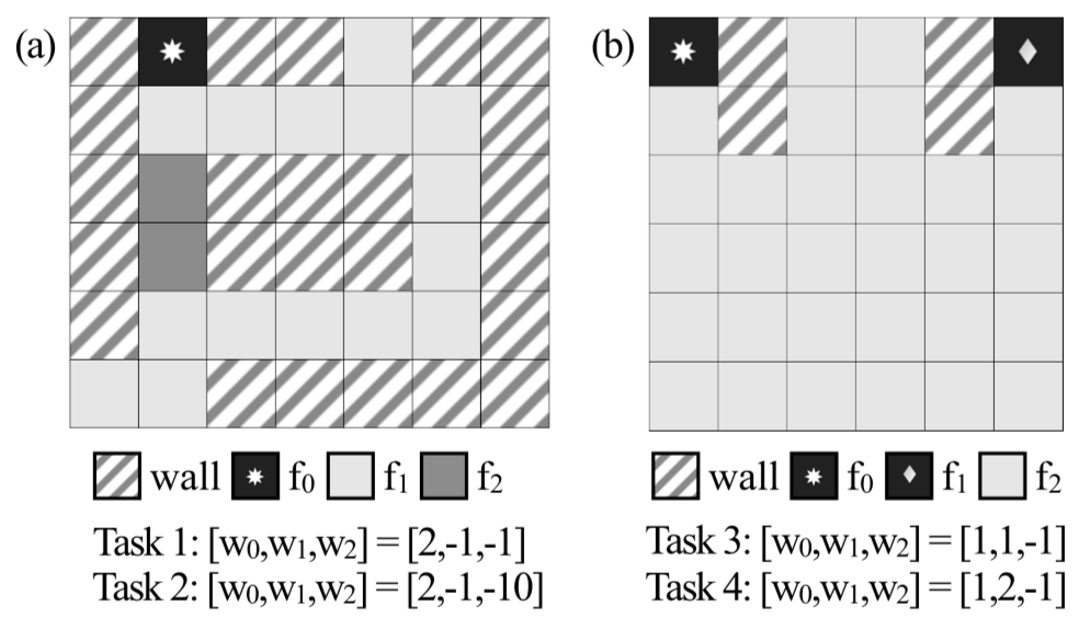
The two grid-worlds used in the paper.
Each of these domains has three features, and furthermore, only one is “active” at a given square in the map, so the vectors are all one-hot. Both domains have two tasks (hence, there are four tasks total), each of which is specified by a particular value of the feature weights. This is the same as specifying a reward function, so the optimal path for an agent may vary.
The paper argues that their algorithm results in the most informative demonstration in the teacher’s set. For the first maze, only one demonstration is necessary to convey each of the two tasks offered: for the second, only two are needed for the two tasks.
From observing example outcomes of the optimal teaching algorithm we get a better intuition about what constitutes an informative demonstration for the learner. A good teacher must show the range of important decision points that are relevant for the task. The most informative trajectories are the ones where the demonstrator makes rational choices among different alternatives, as opposed to those where all possible choices would result in the same behavior.
That the paper’s experiments involve these hand-designed mazes is probably one of the main weaknesses. There’s no way this could extend to high dimensions, when sampling from a hypercube (even if it’s “targeted” in some way, and not sampled naively) would never result in a weight vector that satisfies all the IRL constraints.
To conclude, this AAAI paper, though short and limited in some ways, provided me with a new way of thinking about imitation learning with an active teacher.
Out of curiosity about follow-up, I looked at the Google Scholar of papers that have cited this. Some interesting ones include:
- Cooperative Inverse Reinforcement Learning, NIPS 2016
- Showing versus Doing: Teaching by Demonstration, NIPS 2016
- Enabling Robots to Communicate Their Objectives, RSS 2017
I’m surprised, though, that one of my recent favorite papers, Interpretable and Pedagogical Examples, didn’t cite this one. That one is somewhat similar to this work except it uses more sophisticated Deep Neural Networks within an iterative training procedure, and has far more impressive experimental results. I hope to talk about that paper in a future blog post and to re-implement it in code.