Adversarial Examples and Taxonomies

The following consists of a set of notes that I wrote for students in CS 182/282A about adversarial examples and taxonomies. Before designing these notes, I didn’t know very much about this sub-field, so I had to read some of the related literature. I hope these notes are enough to get the gist of the ideas here. There are two main parts: (1) fooling networks with adversarial examples, and (2) taxonomies of adversarial-related stuff.

Fooling Networks with Adversarial Examples

Two classic papers on adversarial examples in Deep Learning were (Szegedy et al., 2014) followed by (Goodfellow et al., 2015), which were among the first to show that Deep Neural Networks reliably mis-classify appropriately perturbed images that look indistinguishable to “normal” images to the human eye.

More formally, image our deep neural network model $f_\theta$ is parameterized by $\theta$. Given a data point $x$, we want to train $\theta$ so that our $f_\theta(x)$ produces some desirable value. For example, if we have a classification task, then we’ll have a corresponding label $y$, and we would like $f_\theta(x)$ to have an output layer such that the maximal component corresponds to the class index from $y$. Adversarial examples, denoted as $\tilde{x}$, can be written as $\tilde{x} = x + \eta$, where $\eta$ is a small perturbation that causes an imperceptible change to the image, as judged by the naked human eye. Yet, despite the small perturbation, $f_\theta(\tilde{x})$ may behave very different from $f_\theta(x)$, and this has important implications for safety and security reasons if Deep Neural Networks are to be deployed in the real world (e.g., in autonomous driving where $x$ is from a camera sensor).

One of the contributions of (Goodfellow et al., 2015) was to argue that the linear nature of neural networks, and many other machine learning models, makes them vulnerable to adversarial examples. This differed from the earlier claim of (Szegedy et al., 2014) which suspected that it was the complicated nature of Deep Neural Networks that was the source of their vulnerability. (If this sounds weird to you, since neural networks are most certainly not linear, many components behave in a linear fashion, and even advanced layers such as LSTMs and convolutional layers are designed to behave linear or to use linear arithmetic.)

We can gain intuition from looking at a linear model. Consider a weight vector $w$ and an adversarial example $\tilde{x} = x + \eta$, where we additionally enforce the constraint that \(\|\eta\|_\infty < \epsilon\). A linear model $f_w$ might be a simple dot product:

Now, how can we make $w^T\tilde{x}$ sufficiently different from $w^Tx$? Subject to the \(\|\eta\|_\infty \le \epsilon\) constraint, we can set $\eta = \epsilon \cdot {\rm sign}(w)$. That way, all the components in the dot product of $w^T\eta$ are positive, which forcibly increases the difference between $w^Tx$ and $w^T\tilde{x}$.

The equation above contains just a simple linear model, but notice that \(\| \eta \|_\infty\) does not grow with the dimensionality of the problem, because the $L_\infty$-norm takes the maximum over the absolute value of the components, and that must be $\epsilon$ by construction. The change caused by the perturbation, though, grows linearly with respect to the dimension $n$ of the problem. Deep Neural Networks are applied on high dimensional problems, meaning that many small changes can add up to make a large change in the output.

This equation then motivated the the Fast Gradient Sign Method (FGSM) as a cheap and reliable method for generating adversarial examples.¹ Letting $J(\theta, x, y)$ denote the cost (or loss) of training the neural network model, the optimal maximum-norm constrained perturbation $\eta$ based on gradients is

to produce adversarial example $\tilde{x} = x + \eta$. You can alternatively write $\eta = \epsilon \cdot {\rm sign}\left( \nabla_x \mathcal{L}(f_\theta(x), y) \right)$ where $\mathcal{L}$ is our loss function, if that notation is easier to digest.

A couple of comments are in order:

• In (Goodfellow et al., 2015) they set $\epsilon = 0.007$ and were able to fool a GoogLeNet on ImageNet data. That $\epsilon$ is so small that it actually corresponds to the magnitude of the smallest bit of an 8 bit image encoding after GoogLeNet’s conversion to real numbers.

• In the FSGM, the gradient involved is taken with respect to $x$, and not the parameters $\theta$. Therefore, this does not involve changing weights of a neural network, but adjusting the data, similar to what one might do for adjusting an image to “represent” a certain class. Here, our goal is not to generate images that maximally activate the network’s nodes, but to generate adversarial examples while keeping changes to the original image as small as possible.

• It’s also possible to derive a similar “fast gradient” adversarial method based on the $L_2$, rather than $L_\infty$ norm.

• It’s possible to use adversarial networks as part of the training data, in order to make the neural network more robust, such as using the following objective:

  \[\tilde{J}(\theta, x, y) = \alpha J(\theta, x, y) + (1-\alpha) J\left( \theta, x + \epsilon \cdot {\rm sign}(\nabla_x J(\theta,x,y)) \right)\]

  Some promising results were shown in (Goodfellow et al., 2015), which found that it was better than dropout.

• The FGSM requires knowledge of the model $f_\theta$, in order to get the gradient with respect to $x$.

The last point suggests a taxonomy of adversarial methods. That brings us to our next section.

Taxonomies of Adversarial Methods

Two ways of categorizing methods are:

• White-box attacks. The attacker can “look inside” the learning algorithm he/she is trying to fool. The FGSM is a white-box attack method because “looking inside” implies that computing the gradient is possible. I don’t think there is a precise threshold of information that one must have about the model in order for the attack to be characterized as a “white-box attack.” Just view it as when the attacker has more information as compared to a black box attack.

• Black-box attacks. The attacker has no (or little) information about the model he/she is trying to fool. In particular, “looking inside” the learning algorithm is not possible, and this disallows computation of gradients of a loss function. With black boxes, the attacker can still query the model, which might involve providing the model data and then seeing the result. From there the attacker might decide to compute approximate gradients, if gradients are part of the attack.

As suggested above, attack methods may involve querying some model. By “querying,” I mean providing input $x$ to the model $f_\theta$ and obtaining output $f_\theta(x)$. Attacks can be categorized as:

• Zero-query attacks. Those that don’t involve querying the model.

• Query attacks. Those which do involve querying the model. From the perspective of the attacker, it is better to efficiently use few queries, with potentially more queries if their cost is cheap.

There are also two types of adversarial examples in the context of classification:

• Non-Targeted Adversarial Examples: Here, the goal is to mislead a classifier to predict any label other than the ground truth. Formally, given image $x$ with ground truth² $f_\theta(x) = y$, a non-targeted adversarial example can be generated by finding $\tilde{x}$ such that

  \[f_\theta(\tilde{x}) \ne y \quad {\rm subject}\;\;{\rm to} \quad d(x,\tilde{x}) \le B.\]

  where $d(\cdot,\cdot)$ is an appropriate distance metric with a suitable bound $B$.

• Targeted Adversarial Examples: Here, the goal is to mislead a classifier to predict a specific target label. These are harder to generate, because extra work must be done. Not only should the adversarial example reliably cause the classifier to misclassify, it must misclassify to a specific class. This might require finding common perturbations among many different classifiers. We can formalize it as

  \[f_\theta(\tilde{x}) = \tilde{y} \quad {\rm subject}\;\;{\rm to} \quad d(x,\tilde{x}) \le B.\]

  where the difference is that the label $\tilde{y} \ne y$ is specified by the attacker.

There is now an enormous amount of research on Deep Learning and adversarial methods. One interesting research direction is to understand how attack methods transfer among different machine learning models and datasets. For example, given adversarial examples generated for one model, do other models also misclassify those? If this were true, then an obvious strategy that an attacker could do would be to construct a substitute of the black-box model, and generate adversarial instances against the substitute to attack the black-box system.

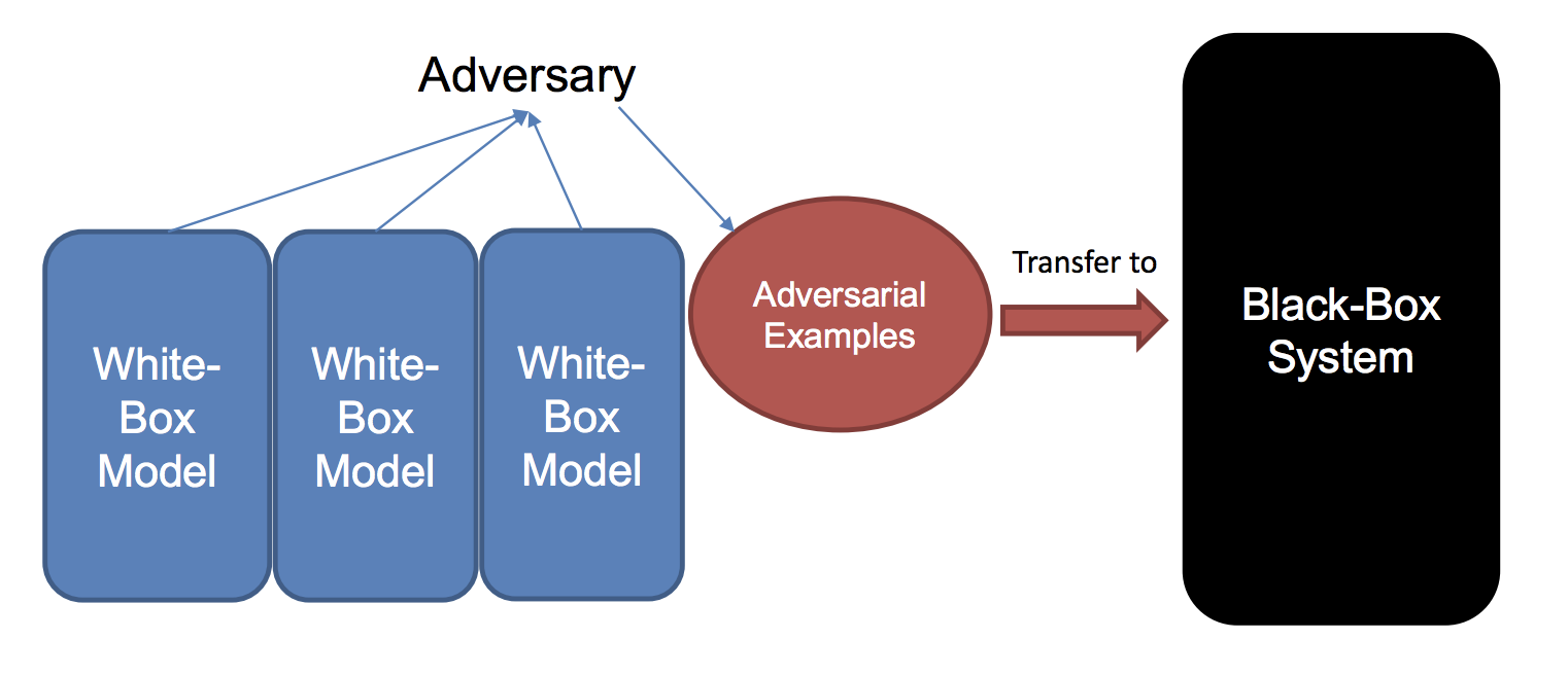
A method proposed in (Liu et al., 2017) for generating adversarial examples using ensembles.

The first large-scale study was reported in (Liu et al., 2017), which studied black-box attacks and transferrability of non-targeted and targeted adversarial examples.³ The highlights of the results were that (a) non-targeted examples are easier to transfer, which we commented earlier above, and (b) it is possible to make even targeted examples more transferrable by using a novel ensemble-based method (sketched in the figure above). The authors applied this on Clarifai.com. This is a black-box image classification system, which we can continually feed images and get outputs. The system in (Liu et al., 2017) demonstrated the ability to transfer targeted adversarial examples generated for models trained on ImageNet to the Clarifai.com system, despite an unknown model, training data, and label set.

Concluding Comments and References

Whew! Hopefully this provides a blog-post bite-sized overview of adversarial examples and related themes. Here are the papers that I cited (and read) while reviewing this content.

1. Christian Szegedy et al., Intriguing Properties of Neural Networks. ICLR, 2014.

2. Ian Goodfellow et al., Explaining and Harnessing AdversarialExamples. ICLR 2015.

3. Yanpei Liu et al., Delving into Transferable Adversarial Examples and Black-box Attacks. ICLR 2017.