DAgger Versus SafeDAgger
The seminal DAgger paper from AISTATS 2011 has had a tremendous impact on machine learning, imitation learning, and robotics. In contrast to the vanilla supervised learning approach to imitation learning, DAgger proposes to use a supervisor to provide corrective labels to counter compounding errors. Part of this BAIR Blog post has a high-level overview of the issues surrounding compounding errors (or “covariate shift”), and describes DAgger as an on-policy approach to imitation learning. DAgger itself — short for Dataset Aggregation — is super simple and looks like this:
- Train \(\pi_\theta(\mathbf{a}_t \mid \mathbf{o}_t)\) from demonstrator data \(\mathcal{D} = \{\mathbf{o}_1, \mathbf{a}_1, \ldots, \mathbf{o}_N, \mathbf{a}_N\}\).
- Run \(\pi_\theta(\mathbf{a}_t \mid \mathbf{o}_t)\) to get an on-policy dataset \(\mathcal{D}_\pi = \{\mathbf{o}_1, \ldots, \mathbf{o}_M\}\).
- Ask a demonstrator to label $\mathcal{D}_\pi$ with actions $\mathbf{a}_t$.
- Aggregate $\mathcal{D} \leftarrow \mathcal{D} \cup \mathcal{D}_{\pi}$ and train again.
with the notation borrowed from Berkeley’s DeepRL course. The training step is usually done via standard supervised learning. The original DAgger paper includes a hyperparameter $\beta$ so that the on-policy data is actually generated with a mixture:
\[\pi = \beta \pi_{\rm supervisor} + (1-\beta) \pi_{\rm agent}\]but in practice I set $\beta=0$, which in this case means all states are generated from the learner agent, and then subsequently labeled from the supervisor.
DAgger is attractive not only in practice but also in terms of theory. The analysis of DAgger relies on mathematical ingredients from regret analysis and online learning, as hinted by the paper title: “A Reduction of Imitation learning and Structured Prediction to No-Regret Online Learning.” You can find some relevant theory in (Kakade and Tewari, NeurIPS 2009).
The Dark Side of DAgger
Now that I have started getting used to reading and reviewing papers in my field, I can more easily understand tradeoffs in algorithms. So, while DAgger is a conceptually simple and effective method, what are its downsides?
- We have to request the supervisor for labels.
- This has to be done for each state the agent encounters when taking steps in an environment.
Practitioners can mitigate these by using a simulated demonstrator, as I have done in some of my robot fabric manipulation work. In fact, I’m guessing this is the norm in machine learning research papers that use DAgger. This is not always feasible, however, and even with a simulated demonstrator, there are advantages to querying less often.
Keeping within the DAgger framework, an obvious solution would be to only request labels for a subset of data points. That’s precisely what the SafeDAgger algorithm, proposed by Zhang and Cho, and presented at AAAI 2017, intends to accomplish. Thus, let’s understand how SafeDAgger works. In the subsequent discussion, I will (generally) use the notation from the SafeDAgger paper.
SafeDAgger
The SafeDAgger paper has a nice high-level summary:
In this paper, we propose a query-efficient extension of the DAgger, called SafeDAgger. We first introduce a safety policy that learns to predict the error made by a primary policy without querying a reference policy. This safety policy is incorporated into the DAgger’s iterations in order to select only a small subset of training examples that are collected by a primary policy. This subset selection significantly reduces the number of queries to a reference policy.
Here is the algorithm:
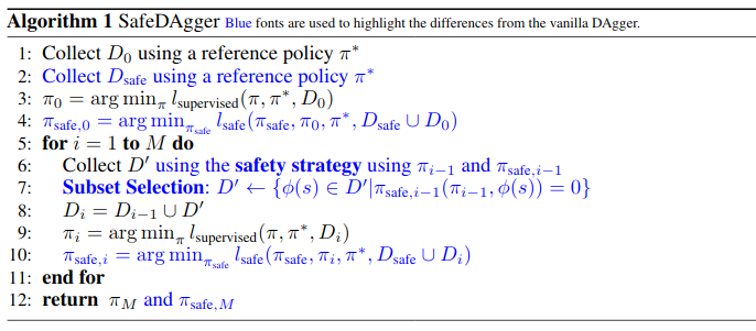
SafeDAgger uses a primary policy $\pi$ and a reference policy \(\pi^*\), and introduces a third policy $\pi_{\rm safe}$, known as the safety policy, which takes in the observation of the state $\phi(s)$ and must determine whether the primary policy $\pi$ is likely to deviate from a reference policy \(\pi^*\) at $\phi(s)$.
A quick side note: I often treat “states” $s$ and “observations” $\phi(s)$ (or $\mathbf{o}$ in my preferred notation) interchangeably, but keep in mind that these technically refer to different concepts. The “reference” policy is also often referred to as a “supervisor,” “demonstrator,” “expert,” or “teacher.”
A very important fact, which the paper (to its credit) repeatedly accentuates, is that because $\pi_{\rm safe}$ is called at each time step to determine if the reference must be queried, $\pi_{\rm safe}$ cannot query \(\pi^*\). Otherwise, there’s no benefit — one might as well dispense with $\pi_{\rm safe}$ all together and query \(\pi^*\) normally for all data points.
The deviation $\epsilon$ is defined with the $L_2$ distance:
\[\epsilon(\pi, \pi^*, \phi(s)) = \| \pi(\phi(s)) - \pi^*(\phi(s)) \|_2^2\]since actions in this case are in continuous land. The optimal safety policy $\pi_{\rm safe}^*$ is:
\[\pi_{\rm safe}^*(\pi, \phi(s)) = \begin{cases} 0, \quad \mbox{if}\; \epsilon(\pi, \pi^*, \phi(s)) > \tau \\ 1, \quad \mbox{otherwise} \end{cases}\]where the cutoff $\tau$ is user-determined.
The real question now is how to train $\pi_{\rm safe}$ from data \(D = \{ \phi(s)_1, \ldots, \phi(s)_N \}\). The training uses the binary cross entropy loss, where the label is “are the two policies taking sufficiently different actions”? For a given dataset $D$, the loss is:
\[\begin{align} l_{\rm safe}(\pi_{\rm safe}, \pi, \pi^*, D) &= - \frac{1}{N} \sum_{n=1}^{N} \pi_{\rm safe}^*(\phi(s)_n) \log \pi_{\rm safe}(\phi(s)_n, \pi) + \\ & (1 - \pi_{\rm safe}^*(\phi(s)_n)) \log(1 - \pi_{\rm safe}(\phi(s)_n, \pi)) \end{align}\]again, here, \(\pi_{\rm safe}^*\) and \((1-\pi_{\rm safe}^*)\) represent ground-truth labels for the cross entropy loss. It’s a bit tricky; the label isn’t something inherent in a training data, but something SafeDAgger artificially enforces to get desired behavior.
Now let’s discuss the control flow of SafeDAgger. The agent collects data by following a safety strategy. Here’s how it works: at every time step, if $\pi_{\rm safe}(\pi, \phi(s)) = 1$, let the usual agent take actions. Otherwise, $\pi_{\rm safe}(\pi, \phi(s)) = 0$ (remember, this function is binary) and the reference policy takes actions. Since this is done at each time step, the reference policy can return control to the agent as soon as it is back into a “safe” state with low action discrepancy.
Also, when the reference policy takes actions, these are the data points that get labeled to produce a subset of data $D’$ that form the input to $l_{\rm safe}$. Hence, the process of deciding which subset of states should be used to query the reference happens during environment interaction time, and is not a post-processing event.
Training happens in lines 9 and 10 of the algorithm, which updates not only the agent $\pi$, but also the safety policy $\pi_{\rm safe}$.
Actually, it’s somewhat strange why the safety policy should help out. If you notice, the algorithm will continually add new data to existing datasets, so while $D_{\rm safe}$ initially produces a vastly different dataset for $\pi_{\rm safe}$ training, in the limit, $\pi$ and $\pi_{\rm safe}$ will be trained on the same dataset. Line 9, which trains $\pi$, will make it so that for all $\phi(s) \in D$, we have \(\pi(\phi(s)) \approx \pi^*(\phi(s))\). Then, line 10 trains $\pi_{\rm safe}$ … but if the training in the previous step worked, then the discrepancies should all be small, and hence it’s unclear why we need a threshold if we know that all observations in the data result in similar actions between \(\pi\) and \(\pi^*\). In some sense $\pi_{\rm safe}$ is learning a support constraint, but it would not be seeing any negative samples. It is somewhat of a philosophical mystery.
Experiments. The paper uses the driving simulator TORCS with a scripted demonstrator. (I have very limited experience with TORCS from an ICRA 2019 paper.)
-
They use 10 tracks, with 7 for training and 3 for testing. The test tracks are only used to evaluate the learned policy (called “primary” in the paper).
-
Using a histogram of squared errors in the data, they decide on $\tau = 0.0025$ as the threshold so that 20 percent of initial training samples are considered “unsafe.”
-
They report damage per lap as a way to measure policy safety, and argue that policies trained with SafeDAgger converge to a perfect, no-damage policy faster than vanilla DAgger. I’m having a hard time reading the plots, though — their “SafeDAgger-Safe” curve in Figure 2 appears to be perfect from the beginning.
-
Experiments also suggest that as the number of DAgger iterations increases, the proportion of time driven by the reference policy decreases.
Future Work? After reading the paper, I had some thoughts about future work directions:
-
First, SafeDAgger is a broadly applicable algorithm. It is not specific to driving, and it should be feasible to apply to other imitation learning problems.
-
Second, the cost is the same for each data point. This is certainly not the case in real life scenarios. Consider context switching: one can request the reference for help in time steps 1, 3, 5, 7, and 9, or it can request the reference for help in times 3, 4, 5, 6, and 7. Both require the same raw number of references, but it seems intuitive in some way that given a fixed budget of time, a reference policy should want a contiguous time step.
-
Finally, one downside strictly from a scientific perspective is that there are no other baseline methods tested other than vanilla DAgger. I wonder if it would be feasible to compare SafeDAgger with an approach such as SHIV from ICRA 2016.
Conclusion
To recap: SafeDAgger follows the DAgger framework, and attempts to reduce the number of queries to the reference/supervisor policy. SafeDAgger predicts the discrepancy among the learner and supervisor. Those states with high discrepancy are those which get queried (i.e., labeled) and used in training.
There’s been a significant amount of follow-up work on DAgger. If I am thinking about trying to reduce supervisor burden, then SafeDAgger is among the methods that come to my mind. Similar algorithms may get increasingly used in machine learning if DAgger-style methods become more pervasive in machine learning research, and in real life.