Twists and Exponential Coordinates

In this post, I build upon my previous one by further investigating fundamental concepts in Murray, Li, and Sastry’s A Mathematical Introduction to Robotic Manipulation. One of the challenges of their book is that there’s a lot of notation, so I first list the important bits here. I then review an example that uses some of this notation to better understand the meaning of twists and exponential coordinates.

Side comment: there is an alternative, more recent robotics book by Frank C. Park and Kevin M. Lynch called Modern Robotics. It’s available online and has its own Wikipedia, and even has some lecture videos! Despite its 2017 publication date, the concepts it describes are very similar to Murray, Li, and Sastry, except that the presentation can be a bit smoother. The notation they use is similar, but with a few exceptions, so be aware of that if you’re reading their book.

Back to our target textbook. Here is relevant notation from Murray, Li, and Sastry:

• The unit vector \(\omega \in \mathbb{R}^3\) specifies a direction of rotation, and \(\theta \in \mathbb{R}\) represents the angle of rotation (in radians).

  An important fact is that any rotation can be represented as rotating by some amount through an axis vector, so we could write rotation matrices \(R\) as functions of \(w\) and \(\theta\), i.e., \(R(\omega, \theta)\). Murray, Li, and Sastry call this “Euler’s Theorem”.

  Note: if you’re familiar with the Product of Exponentials formula, then \(\theta = (\theta_1, \ldots, \theta_J)\), which generalizes to the case when there are \(J\) joints in a robotic arm. Also, \(\theta_i\) doesn’t have to be an angle; it could be a displacement, which would be the case if we had a prismatic joint.

• The cross product matrix \(\hat{\omega}\) satisfies \(\hat{\omega} p = \omega \times p\) for some \(p \in \mathbb{R}^3\), where \(\theta\) indicates the cross product operation. More formally, we have

  \[\hat{\omega} = \begin{bmatrix} 0 & -\omega_3 & \omega_2 \\ \omega_3 & 0 & -\omega_1 \\ -\omega_2 & \omega_1 & 0 \end{bmatrix}\]

  and so \(\hat{\omega}\) is a skew-symmetric matrix, of which the set of those is denoted as \(so(3)\). This is easily verified by explicit computation.

• The matrix exponential \(e^{\hat{\omega} \theta}\) is a \(3\times 3\) matrix in the set \(SO(3)\). In other words, it’s a rotation matrix! We can write it in closed form from Rodrigues’ formula:

  \[e^{\hat{\omega} \theta} = I + \hat{\omega} \sin \theta + \hat{\omega}^2 (1- \cos \theta)\]

  Here’s the relevant mathematical relationship: the exponential map transforms skew-symmetric matrices into orthogonal matrices, and every rotation matrix can be represented as the matrix exponential of some skew-symmetric matrix.

• A twist \(\hat{\xi} \in se(3)\) is defined as the set of \(4\times 4\) matrices parameterized by exponential coordinates \(\xi = (v,\omega)\) s.t. \(v \in \mathbb{R}^3\) and \(\hat{\omega} \in so(3)\). The matrix is written as

  \[\hat{\xi} = \begin{bmatrix} \hat{\omega} & v \\ 0 & 0 \end{bmatrix}\]

  and yes, the last row consists of four zeros. We can derive this matrix from considering rotations about revolute and prismatic joints, where \(\omega\) is the axis of rotation, and \(v\) is the vector describing the translation. (See Section 3.2 in Murry, Li, and Sastry for details.)

  Incidentally, sometimes we call twists as \(\hat{\xi}\theta\), or with the \(\theta\) “attached” to it. We can also do the same for the exponential coordinates.

• The matrix exponential of a twist \(e^{\hat{\xi}\theta}\) represents the relative motion of a rigid body. Hence, if we left-multiply this with a vector, we interpret it as moving the input vector with respect to the same frame. Said another way, we are not changing the “frame of reference” for the input vector.

  Given twist coordinates \((v,\omega)\), we can explicitly construct the RBMs:

  \[e^{\hat{\xi}\theta} = \begin{bmatrix} I & v\theta \\ 0 & 1 \end{bmatrix}\]

  if \(\omega = 0\). This is equivalent to a pure translation. If \(\omega \ne 0\), we have the slightly more complicated formula

  \[e^{\hat{\xi}\theta} = \begin{bmatrix} e^{\hat{\omega}\theta} & (I-e^{\hat{\omega}\theta})(\omega \times v) + \omega \omega^T v \theta \\ 0 & 1 \end{bmatrix} .\]

  Both of the above are elements of \(SE(3)\), so they are rigid body motions. To be clear, you need to construct these from the actual definition of a matrix exponential based on its Taylor series expansion.

Let’s look at the example in the figure below to better understand the above concepts.

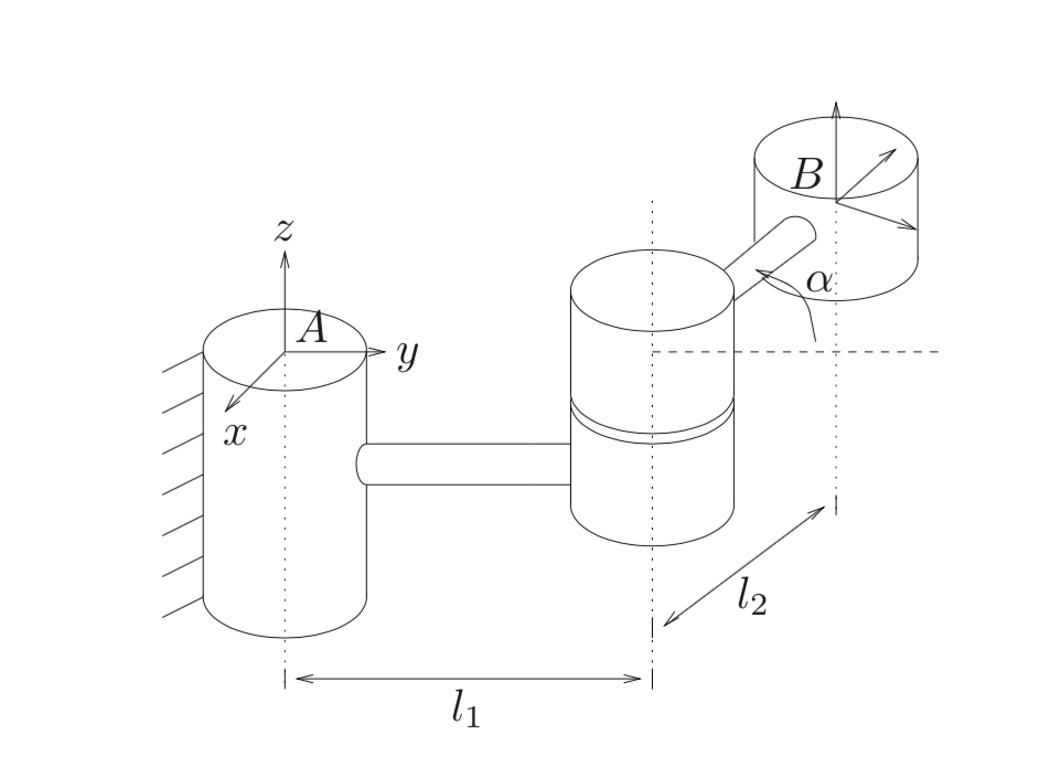
We have inertial frame \(A\) and body frame \(B\). With some pencil and paper, you can show that the RBM from \(B\) to \(A\) is:

which follows the style from my last post: determine the rotation and translation components and then plug them in. Fortunately, the rotation is about the \(z\) axis, so \(R_{ab}\) is easy.

It turns out that every RBM can be expressed as the exponential of some twist \(\xi \in \mathbb{R}^6\). So let’s consider the following:

Given that \(g_{ab} = e^{\hat{\xi} \theta}\) (note \(\hat{\xi}\), not \(\xi\)) and that we know the exact form of \(g_{ab}\), can we compute \(\xi\)?

To do this, we need to compute the components \(v\) and \(\omega\).

• Let’s do \(\omega\) first. From our above equations for \(e^{\hat{\xi}\theta}\) and \(g_{ab}\), we equate components and see that we need

  \[e^{\hat{\omega}\theta} = R_{ab}\]

  We know \(R_{ab}\) corresponds to a rotation matrix about the \(z\)-axis only. This means \(\omega = (0,0,1)\). We also simply set \(\alpha = \theta\).

• Now consider \(v\). Once again, we equate components from both sides to get

  \[p_{ab} = \begin{bmatrix} (I-e^{\hat{\omega}\theta})(\omega \times v) + \omega \omega^T v \theta \end{bmatrix} = \begin{bmatrix} (I-e^{\hat{\omega}\theta})\hat{\omega} + \omega \omega^T \theta \end{bmatrix} v\]

  This is the standard “solve for \(x\) in \(Ax=b\)” problem that you saw in linear algebra classes. Solving for \(v\), we get \(v = (\frac{l_1-l_2}{2}, \frac{(l_1+l_2)\sin\alpha}{2(1-\cos\alpha)}, 0)\).

We conclude that our exponential coordinates which generated \(g_{ab}\) are

assuming that \(\alpha \ne 0\)