Interpretable and Pedagogical Examples
In my last post, I discussed a paper on algorithmic teaching. I mentioned in the last paragraph that there was a related paper, Interpretable and Pedagogical Examples, that I’d be interested in reading in detail. I was able to do that sooner than expected, so naturally, I decided to blog about it. A few months ago, OpenAI had a blog post discussing the contribution and ramifications of the paper, so I’m hoping to focus more on stuff they didn’t cover to act as a complement.
This paper is currently “only” on arXiv as it was rejected from ICLR 2018 — not due to lack of merit, it seems, but because the authors had their names on the manuscript, violating the double-blind nature of ICLR. I find it quite novel, though, and hope it finds a home somewhere in a conference.
There are several contributions of this over prior work in machine teaching and the like. First, they use deep recurrent neural networks for both the student and the teacher. Second and more importantly, they show that with iterative — not joint — training, the teacher will teach using an interpretable strategy that matches human intuition, and which furthermore is efficient in conveying concepts with the fewest possible samples (hence, “pedagogical”). This paper focus on teaching by example, but there are other ways to teach, such as using pairwise comparisons as in this other OpenAI paper.
How does this work? We consider a two-agent environment with a student \(\mathbf{S}\) and a teacher \(\mathbf{T}\), both of which are parameterized by deep recurrent neural networks \(\theta_{\mathbf{S}}\) and \(\theta_{\mathbf{T}}\), respectively. The setting also involves a set of concepts \(\mathcal{C}\) (e.g., different animals) and examples \(\mathcal{E}\) (e.g., images of those animals).
The student needs to map a series of \(K\) examples to concepts. At each time step \(t\), it guesses the concept \(\hat{c}\) that the teacher is trying to convey. The teacher, at each time step, takes in \(\hat{c}\) along with the concept it is trying to convey, and must output an example that (ideally) will make \(\hat{c}\) “closer” to \(c\). Examples may be continuous or discrete.
As usual, to train \(\mathbf{S}\) and \(\mathbf{T}\), it is necessary to devise an appropriate loss function \(\mathcal{L}\). In this paper, the authors chose to have \(\mathcal{L}\) be a function from \(\mathcal{C}\times \mathcal{C} \to \mathbb{R}\) where the input is the true concept and the student’s concept after the \(K\) examples. This is applied to both the student and teacher; they use the same loss function and are updated via gradient descent. Intuitively, this makes sense: both the student and teacher want the student to know the teacher’s concept. The loss is usually the \(L_2\) (continuous) or the cross-entropy (discrete).
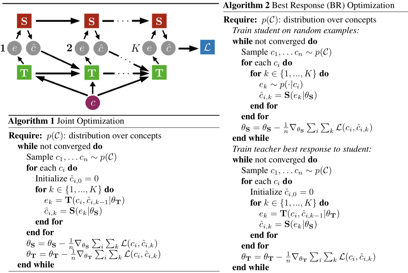
A collection of important aspects from the paper "Interpretable and Pedagogical
Examples." Top left: a visualization of the training process. Bottom left: joint
training baseline which should train the student but not create interpretable
teaching strategies. Right: iterative training procedure which should create
interpretable teaching strategies.
The figure above includes a visualization of the training process. It also includes both the joint and iterative training procedures. The student’s function is written as \(\mathbf{S}(e_k | \theta_{\mathbf{S}})\), and this is what is used to produce the next concept. The authors don’t explicitly pass in the previous examples or the student’s previously predicted concepts (the latter of which would make this an “autoregressive” model) because, presumably, the recurrence means the hidden layers implicitly encode the essence of this prior information. A similar thing is seen with how one writes the teacher’s function: \(\mathbf{T}(c_i, \hat{c}_{i,k-1} | \theta_{\mathbf{T}})\).
The authors argue that joint training means the teacher and student will “collude” and produce un-interpretable teaching, while iterative training lets them obtain interpretable teaching strategies. Why? They claim:
The intuition behind separating the optimization into two steps is that if \(\mathbf{S}\) learns an interpretable learning strategy in Step 1, then \(\mathbf{T}\) will be forced to learn an interpretable teaching strategy in Step 2. The reason we expect \(\mathbf{S}\) to learn an “interpretable” strategy in Step 1 is that it allows \(\mathbf{S}\) to learn a strategy that exploits the natural mapping between concepts and examples.
I think the above reason boils down to the fact that the teacher “knows” the true concepts \(c_1,\ldots,c_n\) in the minibatch of concepts above, and those are fixed throughout the student’s training portion. Of course, this would certainly be easier to understand after implementing it in code!
The experimental results are impressive and cover a wide range of scenarios:
-
Rule-Based: this is the “rectangle game” from cognitive science, where teachers provide points within a rectangle, and the student must guess the boundary. The intuitive teaching strategy would be to provide two points at opposite corners.
-
Probabilistic: the teacher must teach a bimodal mixture of Gaussians distribution, and the intuitive strategy is to provide points at the two modes (I assume, based on the relative weights of the two Gaussians).
-
Boolean: how does the teacher teach an object property, when objects may have multiple properties? The intuitive strategy is to provide two points where, of all the properties in the provided/original dataset, the only one that the two have in common is what the teacher is teaching.
-
Hierarchical: how does a teacher teach a hierarchy of concepts? The teacher learns the intuitive strategy of picking two examples whose lowest common ancestor is the concept node. Here, the authors use images from a “subtree” of ImageNet and use a pre-trained Res-Net to cut the size of all images to be vectors in \(\mathbb{R}^{2048}\).
For the first three above, the loss is \(\mathcal{L}(c,\hat{c}) = \|c-\hat{c}\|_2^2\), whereas the fourth problem setting uses the cross entropy.
There is also evaluation that involves human subjects, which is the second definition of “interpretability” the authors invoke: how effective is \(\mathbf{T}\)’s strategy at teaching humans? They do this using the probabilistic and rule-based experiments.
Overall, this paper is enjoyable to read, and the criticism that I have is likely beyond the scope that any one paper can cover. One possible exception: understanding the neural network architecture and training. The architecture, for instance, is not specified anywhere. Furthermore, some of the training seemed excessively hand-tuned. For example, the authors tend to train using \(X\) examples for \(K\) iterations but I wonder if these needed to be tuned.
I think I would like to try implementing this algorithm (using PyTorch to boot!), since it’s been a while since I’ve seriously tried replicating a prior result.