Actor-Critic Methods: A3C and A2C

Actor-critic methods are a popular deep reinforcement learning algorithm, and having a solid foundation of these is critical to understand the current research frontier. The term “actor-critic” is best thought of as a framework or a class of algorithms satisfying the criteria that there exists parameterized actors and critics. The actor is the policy \(\pi_{\theta}(a \mid s)\) with parameters \(\theta\) which conducts actions in an environment. The critic computes value functions to help assist the actor in learning. These are usually the state value, state-action value, or advantage value, denoted as \(V(s)\), \(Q(s,a)\), and \(A(s,a)\), respectively.

I suggest that the most basic actor-critic method (beyond the tabular case) is vanilla policy gradients with a learned baseline function.¹ Here’s an overview of this algorithm:

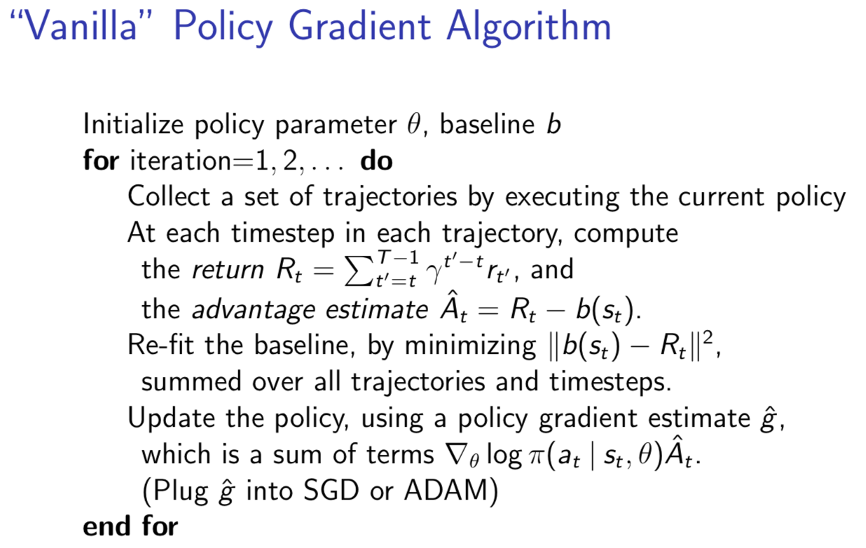
The basic vanilla policy gradients algorithm. Credit: John Schulman.

I also reviewed policy gradients in an older blog post, so I won’t repeat the details.² I used expected values in that post, but in practical implementations, you’ll just take the saved rollouts to approximate the expectation as in the image above. The main point to understand here is that an unbiased estimate of the policy gradient can be done without the learned baseline \(b(s_t)\) (or more formally, \(b_{\theta_C}(s_t)\) for parameters \(\theta_C\)) by just using \(R_t\), but this estimate performs poorly in practice. Hence why, people virtually always apply a baseline.

My last statement is somewhat misleading. Yes, people apply learned baseline functions, but I would argue that the more important thing is to ditch vanilla policy gradients all together and use a more sophisticated framework of actor critic methods, called A3C and popularized from the corresponding DeepMind ICML 2016 paper.³ In fact, when people refer to “actor-critic” nowadays, I think this paper is often the associated reference, and one can probably view it as the largest or most popular subset of actor-critic methods. This is despite how the popular DDPG algorithm is also an actor-critic method, perhaps because its is more commonly thought of as the continuous control analogue of DQN, which isn’t actor-critic as the critic (Q-network) suffices to determine the policy; just take a softmax and pick the action maximizing the Q-value.

A3C stands for Asynchronous Advantage Actor Critic. At a high level, here’s what the name means:

• Asynchronous: because the algorithm involves executing a set of environments in parallel (ideally, on different cores⁴ in a CPU) to increase the diversity of training data, and with gradient updates performed in a Hogwild! style procedure. No experience replay is needed, though one could add it if desired (this is precisely the ACER algorithm).

• Advantage: because the policy gradient updates are done using the advantage function; DeepMind specifically used \(n\)-step returns.

• Actor: because this is an actor-critic method which involves a policy that updates with the help of learned state-value functions.

You can see what the algorithm looks like mathematically in the paper and in numerous blog posts online. For me, a visual diagram helps. Here’s what I came up with:

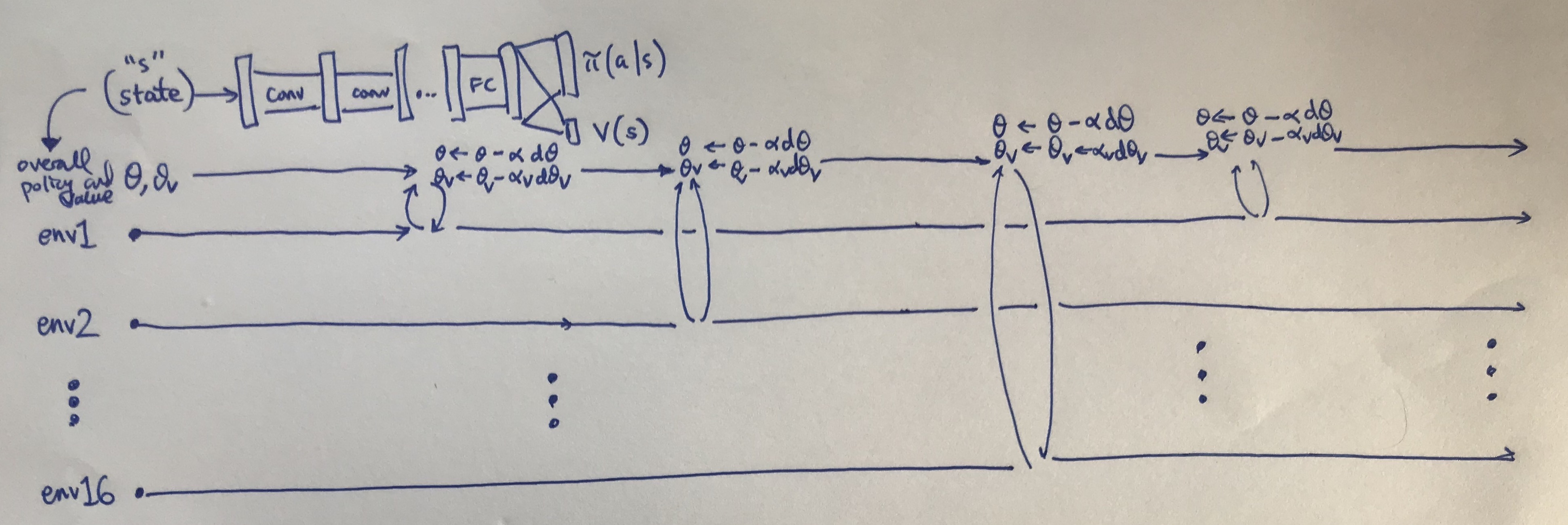My visualization of how A3C works.

A few points:

• I’m using 16 environments in parallel, since that’s what DeepMind used. I suppose I could use close to this in modern machines since many CPUs have four or six cores, and with hyperthreading we get double that. Of course, it might be easier to simply use Amazon Web Services … and incidentally, no GPU is needed.

• I share the value function and the policy in the same way DeepMind did, but for generality I keep the gradient updates separate for \(\theta\) (the policy) and \(\theta_v\) (the value function) and have respective learning rates \(\alpha\) and \(\alpha_v\). In TensorFlow code, I would watch out for the variables that my optimizers update.

• The policy has an extra entropy bonus regularizer that is embedded in the \(d\theta\) term to encourage exploration.

• The updates are done in Hogwild! fashion, though nothing I drew in the figure above actually shows that, since it assumes that different threads reached their “update point” at different times and update separately. Hogwild! would apply when two or more threads call a gradient update to the shared parameter simultaneously, raising the possibility of one thread overwriting another. This shouldn’t happen too often, since there’s only 16 threads — my intuition is that it’d be a lot worse with orders of magnitude more threads — but the point is even if they do, things should be fine in the long run.

• The advantage is computed using \(n\)-step returns with something known as the forward view, rather than the backward view, as done with eligibility traces. If you are unfamiliar with “eligibility traces” then I recommend reading Sutton and Barto’s online reinforcement learning textbook.

I’ll expand on the last point a bit, drawing upon some math from my older blog post about Generalized Advantage Estimation. The point here is to use more than just the one-step return from the standard Q-value definition. Despite the addition of more time steps, we still get an approximation of the advantage function (and arguably a better one). At each time step, we can accumulate a gradient, and at the designated stopping point, that thread pushes the updates to the central parameter server. Even though I’m sure all the thread’s gradients are highly correlated, the different threads in use should suffice for a diverse set of gradients.

To be clear about this, for some interval where the thread’s agent takes steps, we get rewards \(r_1, r_2, \ldots, r_k\), where upon reaching the \(k\)-th step, the agent stopped, either due to reaching a terminal state or because it’s reached the human-designated maximum number of steps before an update. Then, for the advantage estimate, we go backwards in time to accumulate the discounted reward component. For the last time step, we’d get

for the penultimate step, we’d get:

then the next:

and so on. See the pseudocode in the A3C paper if this is not clear.

The rewards were already determined from executing trajectories in the environment, and by summing them this way, we get the empirical advantage estimate. The value function which gets subtracted has subscripts that match the advantage (because \(A(s,a) = Q(s,a)-V(s)\)), but not the value function used for the \(n\)-step return. Incidentally, that value will often be zero, and it should be zero if this trajectory ended due to a terminal state.

Now let’s talk about A2C: Advantage Actor Critic. Given the name (A2C vs A3C) why am I discussing A2C after A3C if it seems like it might be simpler? Ah, it turns out that (from OpenAI):

After reading the paper, AI researchers wondered whether the asynchrony led to improved performance (e.g. “perhaps the added noise would provide some regularization or exploration?“), or if it was just an implementation detail that allowed for faster training with a CPU-based implementation.

As an alternative to the asynchronous implementation, researchers found you can write a synchronous, deterministic implementation that waits for each actor to finish its segment of experience before performing an update, averaging over all of the actors.

Thus, think of the figure I have above, but with all 16 of the threads waiting until they all have an update to perform. Then we average gradients over the 16 threads with one update to the network(s). Indeed, this should be more effective due to larger batch sizes.

In the OpenAI baselines repository, the A2C implementation is nicely split into four clear scripts:

• The main call, run_atari.py, in which we supply the type of policy and learning rate we want, along with the actual (Atari) environment. By default, the code sets the number of CPUs (i.e., number of environments) to 16 and then creates a vector of 16 standard gym environments, each specified by a unique integer rank. I think the rank is mostly for logging purposes, as they don’t seem to be using mpi4py for the Atari games. The environments and CPUs utilize the Python multiprocessing library.

• Building policies (policies.py), for the agent. These build the TensorFlow computational graphs and use CNNs or LSTMs as in the A3C paper.

• The actual algorithm (a2c.py), with a learn method that takes the policy function (from policies.py) as input. It uses a Model class for the overall model and a Runner class to handle the different environments executing in parallel. When the runner takes a step, this performs a step for each of the 16 environments.

• Utilities (utils.py), since helper and logger methods help make any modern DeepRL algorithm easier to implement.

The environment steps are still a CPU-bound bottleneck, though. Nonetheless, I think A2C is likely my algorithm of choice over A3C for actor-critic based methods.

Update: as of September 2018, the baselines code has been refactored. In particular, there is now an algorithm-agnostic run script that gets called, and they moved some of the policy-building (i.e., neural network building) code into the common sub-package. Despite the changes, the general structure of their A2C algorithm is consistent with what I’ve written above. Feel free to check out my other blog post which describes some of these changes in more detail.