On OpenAI Baselines Refactored and the A2C Code
OpenAI, a San Francisco nonprofit organization, has been in the news for a number of reasons, such as when their Dota2 AI system was able to beat a competitive semi-professional team, and when they trained a robotic hand to have unprecedented dexterity, and in various contexts about their grandiose mission of founding artificial general intelligence. It’s safe to say that such lofty goals are characteristic of an Elon Musk-founded company (er, nonprofit). I find their technical accomplishments impressive thus far, and hope that OpenAI can continue their upward trajectory in impact. What I’d like to point out in this blog post, though, is that I don’t actually find their Dota2 system, their dexterous hand, or other research products to be their most useful or valuable contribution to the AI community.
I think OpenAI’s open-source baselines code repository wins the prize of their most important product. You can see an announcement in a blog post from about 1.5 years ago, where they correctly point out that reinforcement learning algorithms, while potentially simple to describe and outline in mathematical notation, are surprisingly hard to implement and debug. I have faced my fair share of issues in implementing reinforcement learning algorithms, and it was a relief to me when I found out about this repository. If other AI researchers base their code on this repository, then it makes it far easier to compare and extend algorithms, and far easier to verify correctness (always a concern!) of research code.
That’s not to say it’s been a smooth ride. Far from it, in fact. The baselines repository has been notorious for being difficult to use and extend. You can find plenty of complaints and constructive criticism on the GitHub issues and on reddit (e.g., see this thread).
The good news is that over the last few months — conveniently, when I was distracted with ICRA 2019 — they substantially refactored their code base.
While the refactoring is still in progress for some of the algorithms (e.g., DDPG, HER, and GAIL seem to be following their older code), the shared code and API that different algorithms should obey is apparent.
First, as their README states, algorithms should now be run with the following command:
python -m baselines.run --alg=<name of the algorithm> \
        --env=<environment_id> [additional arguments]
The baselines.run is a script shared across algorithms that handles the
following tasks:
-
It processes command line arguments and handles “ranks” for MPI-based code. MPI is used for algorithms that require multiple processes for parallelism.
-
It runs the training method, which returns a
modeland anenv.-
The training method needs to first fetch the learning function, along with its arguments.
-
It does this by treating the algorithm input (e.g.,
'a2c'in string form) as a python module, and then importing alearnmethod. Basically, this means in a sub-directory (e.g.,baselines/a2c) there needs to be a python script of the same name (which would bea2c.pyin this example) which defines alearnmethod. This is the main “entry point” for all refactored algorithms. -
After fetching the learning function, the code next searches to see if there are any default arguments provided. For A2C it looks like it lacks a
defaults.pyfile, so there are no defaults specified outside of thelearnmethod. If there was such a file, then the arguments indefaults.pyoverride those inlearn. In turn,defaults.pyis overriden by anything that we write on the command line. Whew, got that?
-
-
Then it needs to build the environment. Since parallelism is so important for algorithms like A2C, this often involves creating multiple environments of the same type, such as creating 16 different instantiations of the Pong game. (Such usage also depends on the environment type: whether it’s atari, retro, mujoco, etc.)
-
Without any arguments for
num_env, this will often default to the number of CPUs on the system from runningmultiprocessing.cpu_count(). For example, on my Ubuntu 16.04 machine with a Titan X (Pascal) GPU, I have 8 CPUs. This is also the value I see when runninghtop. Technically, my processor only supports 4 CPUs, but the baseline code “sees” 8 CPUs due to hyperthreading. -
They use the
SubprocVecEnvclasses for making multiple environments of the same type. In particular, it looks like it’s called as:SubprocVecEnv([make_env(i + start_index) for i in range(num_env)])from
make_vec_envinbaselines/common/cmd_util.py, where each environment is created with its own ID, and themake_envmethod further creates a random seed based on the MPI rank. This is a list of OpenAI gym environments, as one would expect. -
The current code comments in
SubprocVecEnvsuccinctly describe why this class exists:VecEnv that runs multiple environments in parallel in subproceses and communicates with them via pipes. Recommended to use when num_envs > 1 and step() can be a bottleneck.
It makes sense to me. Otherwise, we’d need to sequentially iterate through a bunch of
step()functions in a list — clearly a bottleneck in the code. Bleh! There’s a bunch of functionality that should look familiar to those who have used the gym library, except it considers the combination of all the environments in the list. -
In A2C, it looks like the
SubprocVecEnvclass is further passed as input to theVecFrameStackclass, so it’s yet another wrapper. Wrappers, wrappers, and wrappers all day, yadda yadda yadda. This means it will call theSubprocVecEnv’s methods, such asstep_wait(), and process the output (observations, rewards, etc.) as needed and then pass them to an end-algorithm like A2C with the same interface. In this case, I think the wrapper provides functionality to stack the observations so that they are all in one clean numpy array, rather than in an ugly list, but I’m not totally sure.
-
-
Then it loads the network used for the agent’s policy. By default, this is the Nature CNN for atari-based environments, and a straightforward (input-64-64-output) fully connected network otherwise. The TensorFlow construction code is in
baselines.common.models. The neural networks are not built until the learning method is subsequently called, as in the next bullet point: -
Finally, it runs the learning method it acquired earlier. Then, after training, it returns the trained model. See the individual algorithm directories for details on their
learnmethod.-
In A2C, for instance, one of the first things the
learnmethod does is to build the policy. For details, seebaselines/common/policies.py. -
There is one class there,
PolicyWithValue, which handles building the policy network and seamlessly integrates shared parameters with a value function. This is characteristic of A2C, where the policy and value functions share the same convolutional stem (at least for atari games) but have different fully connected “branches” to complete their individual objectives. When running Pong (see commands below), I get this as the list of TensorFlow trainable parameters:<tf.Variable 'a2c_model/pi/c1/w:0' shape=(8, 8, 4, 32) dtype=float32_ref> <tf.Variable 'a2c_model/pi/c1/b:0' shape=(1, 32, 1, 1) dtype=float32_ref> <tf.Variable 'a2c_model/pi/c2/w:0' shape=(4, 4, 32, 64) dtype=float32_ref> <tf.Variable 'a2c_model/pi/c2/b:0' shape=(1, 64, 1, 1) dtype=float32_ref> <tf.Variable 'a2c_model/pi/c3/w:0' shape=(3, 3, 64, 64) dtype=float32_ref> <tf.Variable 'a2c_model/pi/c3/b:0' shape=(1, 64, 1, 1) dtype=float32_ref> <tf.Variable 'a2c_model/pi/fc1/w:0' shape=(3136, 512) dtype=float32_ref> <tf.Variable 'a2c_model/pi/fc1/b:0' shape=(512,) dtype=float32_ref> <tf.Variable 'a2c_model/pi/w:0' shape=(512, 6) dtype=float32_ref> <tf.Variable 'a2c_model/pi/b:0' shape=(6,) dtype=float32_ref> <tf.Variable 'a2c_model/vf/w:0' shape=(512, 1) dtype=float32_ref> <tf.Variable 'a2c_model/vf/b:0' shape=(1,) dtype=float32_ref>There are separate policy and value branches, which are shown in the bottom four lines above. There are six actions in Pong, which explains why one of the dense layers has shape 512x6. Their code technically exposes two different interfaces to the policy network to handle stepping during training and testing, since these will in general involve different batch sizes for the observation and action placeholders.
-
The A2C algorithm uses a
Modelclass to define various TensorFlow placeholders and the computational graph, while theRunnerclass is for stepping in the (parallel) environments to generate experiences. Within thelearnmethod (which is what actually creates the model and runner), for each update step, the code is remarkably simple: call the runner to generate batches, call the train method to update weights, print some logging statistics, and repeat. Fortunately, the runner returns observations, actions, and other stuff in numpy form, making it easy to print and inspect. -
Regarding the batch size: there is a parameter based on the number of CPUs (e.g., 8). That’s how many environments are run in parallel. But there is a second parameter,
nsteps, which is 5 by default. This is how many steps the runner will execute for each minibatch. The highlights of the runner’srunmethod looks like this:for n in range(self.nsteps): actions, values, states, _ = self.model.step( self.obs, S=self.states, M=self.dones) # skipping a bunch of stuff ... obs, rewards, dones, _ = self.env.step(actions) # skipping a bunch of stuff ...The model’s
stepmethod returns actions, values and states for each of the parallel environments, which is straightforward to do since it’s a batch size in the network’s forward pass. Then, theenvclass can step in parallel using MPI and the CPU. All of these results are combined fornstepswhich multiplies an extra factor to the batch size. Then the rewards are computed based on thensteps-step returns, which is normally 5. Indeed, from checking the original A3C paper, I see that DeepMind used 5-step returns. Minor note: technically 5 is the maximum “step-return”: the last time step uses the 1-step return, the penultimate time step uses the 2-step return, and so on. It can be tricky to think about.
-
-
-
At the end, it handles saving and visualizing the agent, if desired. This uses the
stepmethod from both theModeland theenv, to handle parallelism. TheModelstep method directly calls thePolicyWithValue’sstepfunction. This exposes the value function, which allows us to see what the network thinks regarding expected return.
Incidentally, I have listed the above in order of code logic, at least as of today’s baselines code. Who knows what will happen in a few months?
Since the code base has been refactored, I decided to run a few training scripts to see performance. Unfortunately, despite the refactoring, I believe the DQN-based algorithms still are not correctly implemented. I filed a GitHub issue where you can check out the details, and suffice to say, this is a serious flaw in the baselines repository.
So for now, let’s not use DQN. Since A2C seems to be working, let us go ahead and test that. I decided to run the following command line arguments:
python -m baselines.run --alg=a2c --env=PongNoFrameskip-v4 --num_timesteps=2e7 \
        --num_env=2  --save_path=models/a2c_2e7_02cpu

python -m baselines.run --alg=a2c --env=PongNoFrameskip-v4 --num_timesteps=2e7 \
        --num_env=4  --save_path=models/a2c_2e7_04cpu

python -m baselines.run --alg=a2c --env=PongNoFrameskip-v4 --num_timesteps=2e7 \
        --num_env=8  --save_path=models/a2c_2e7_08cpu

python -m baselines.run --alg=a2c --env=PongNoFrameskip-v4 --num_timesteps=2e7 \
        --num_env=16 --save_path=models/a2c_2e7_16cpu
Yes, I know my computer has only 8 CPUs but I am running with 16. I’m not actually sure how this works, maybe each CPU has to deal with two processes sequentially? Heh.
When you run these commands, it (in the case of 16 environments) creates the following output in the automatically-created log directory:
daniel@takeshi:/tmp$ ls -lh openai-2018-09-26-16-06-58-922448/
total 568K
-rw-rw-r-- 1 daniel daniel 7.7K Sep 26 17:33 0.0.monitor.csv
-rw-rw-r-- 1 daniel daniel 7.7K Sep 26 17:33 0.10.monitor.csv
-rw-rw-r-- 1 daniel daniel 7.7K Sep 26 17:33 0.11.monitor.csv
-rw-rw-r-- 1 daniel daniel 7.7K Sep 26 17:33 0.12.monitor.csv
-rw-rw-r-- 1 daniel daniel 7.7K Sep 26 17:33 0.13.monitor.csv
-rw-rw-r-- 1 daniel daniel 7.7K Sep 26 17:33 0.14.monitor.csv
-rw-rw-r-- 1 daniel daniel 7.6K Sep 26 17:33 0.15.monitor.csv
-rw-rw-r-- 1 daniel daniel 7.7K Sep 26 17:33 0.1.monitor.csv
-rw-rw-r-- 1 daniel daniel 7.7K Sep 26 17:33 0.2.monitor.csv
-rw-rw-r-- 1 daniel daniel 7.7K Sep 26 17:33 0.3.monitor.csv
-rw-rw-r-- 1 daniel daniel 7.7K Sep 26 17:33 0.4.monitor.csv
-rw-rw-r-- 1 daniel daniel 7.8K Sep 26 17:33 0.5.monitor.csv
-rw-rw-r-- 1 daniel daniel 7.7K Sep 26 17:33 0.6.monitor.csv
-rw-rw-r-- 1 daniel daniel 7.8K Sep 26 17:33 0.7.monitor.csv
-rw-rw-r-- 1 daniel daniel 7.7K Sep 26 17:33 0.8.monitor.csv
-rw-rw-r-- 1 daniel daniel 7.8K Sep 26 17:33 0.9.monitor.csv
-rw-rw-r-- 1 daniel daniel 333K Sep 26 17:33 log.txt
-rw-rw-r-- 1 daniel daniel  95K Sep 26 17:33 progress.csv
Clearly, there is one monitor.csv for each of the 16 environments, which
contains the corresponding environment’s episode rewards (and not the other 15).
The log.txt is the same as the standard output, and progress.csv records
the log’s stats.
Using this python script, I plotted the results. They are shown in the image below, which you can expand in a new window to see the full size.
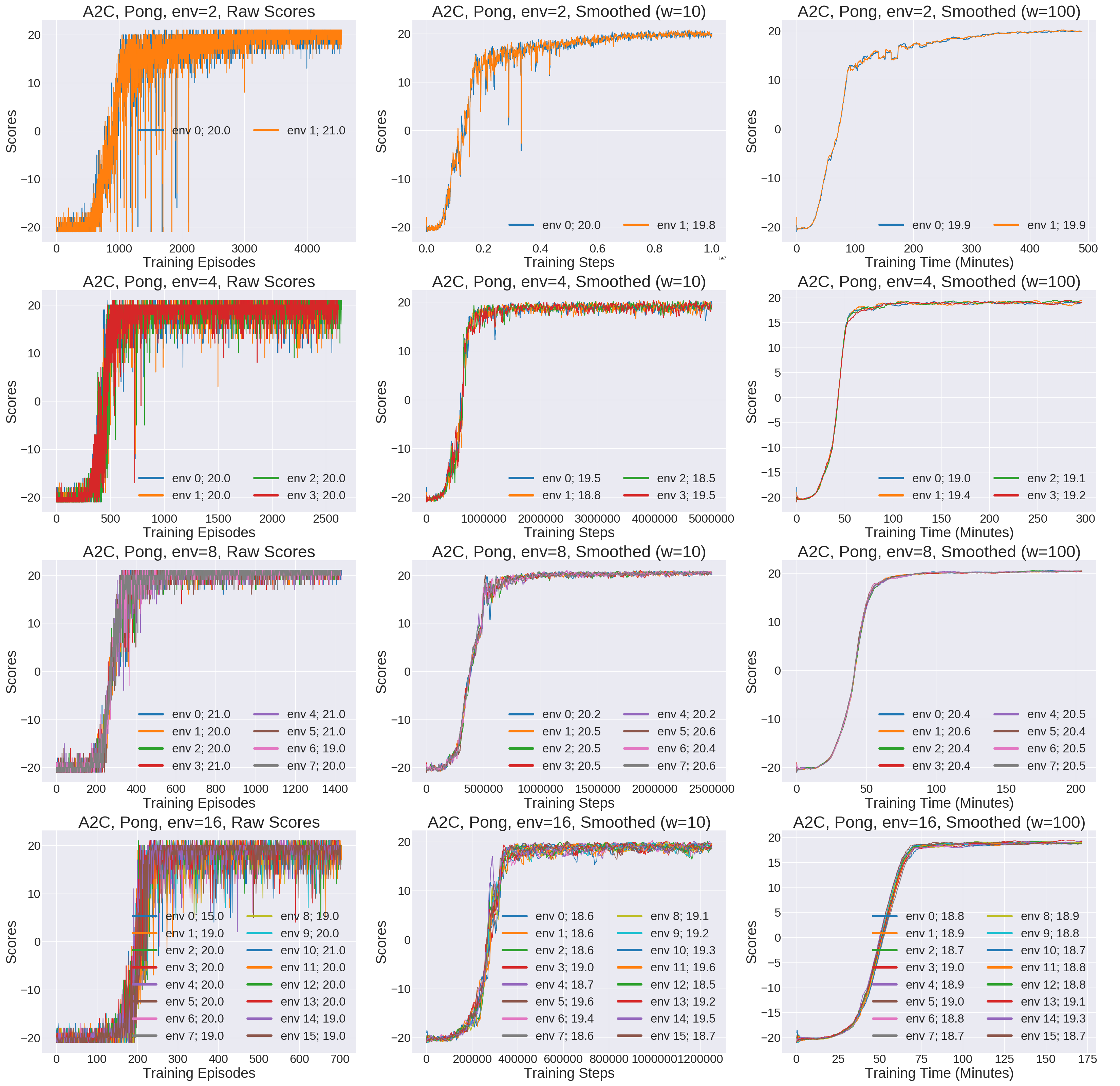
Results of the A2C commands. Each row corresponds to using a different number of
environments (2, 4, 8, or 16) in A2C, and each column corresponds to some
smoothing setting for the score curves, and some option for the x-axis
(episodes, steps, or time).
It seems like running with 8 environments results in the best game scores, with the final values for all 8 surpassing 20 points. The other three settings look like they need a little more training to get past 20. Incidentally, the raw scores (left column) are noisy, so the second and third column represent smoothing over a window of 10 and 100 episodes, respectively.
The columns also report scores as a function of different items we might care about: training episodes, training steps, or training time (in minutes). The x-axis values vary across the different rows, because the 2e7 steps limit considers the combination of all steps in the parallel environments. For example, the 16 environment case ran in 175 minutes (almost 3 hours). Interestingly enough, the speedup over the 8 environment case is smaller than one might expect, perhaps because my computer only has 8 CPUs. There is, fortunately, a huge gap in speed between the 8 and 4 settings.
Whew! That’s all for now. I will continue checking the baselines code repository for updates. I will also keep trying out more algorithms to check for correctness and to understand usage. Thanks, OpenAI, for releasing such an incredibly valuable code base!