Offline (Batch) Reinforcement Learning: A Review of Literature and Applications
Reinforcement learning is a promising technique for learning how to perform tasks through trial and error, with an appropriate balance of exploration and exploitation. Offline Reinforcement Learning, also known as Batch Reinforcement Learning, is a variant of reinforcement learning that requires the agent to learn from a fixed batch of data without exploration. In other words, how does one maximally exploit a static dataset? The research community has grown interested in this in part because larger datasets are available that might be used to train policies for physical robots. Exploration with a physical robot may risk damage to robot hardware or surrounding objects. In addition, since offline reinforcement learning disentangles exploration from exploitation, it can help provide standardized comparisons of the exploitation capability of reinforcement learning algorithms.
Offline reinforcement learning, henceforth Offline RL, is closely related to imitation learning (IL) in that the latter also learns from a fixed dataset without exploration. However, there are several key differences.
-
Offline RL algorithms (so far) have been built on top of standard off-policy Deep Reinforcement Learning (Deep RL) algorithms, which tend to optimize some form of a Bellman equation or TD difference error.
-
Most IL problems assume an optimal, or at least a high-performing, demonstrator which provides data, whereas Offline RL may have to handle highly suboptimal data.
-
Most IL problems do not have a reward function. Offline RL considers rewards, which furthermore can be processed after-the-fact and modified.
-
Some IL problems require the data to be labeled as expert versus non-expert. Offline RL does not make this assumption.
I preface the IL descriptions with “some” and “most” because there are exceptions to every case and that the line between methods is not firm, as I emphasized in a blog post about combining IL and RL.
Offline RL is therefore about deriving the best policy possible given the data. This gives us the hope of out-performing the demonstration data, which is still often a difficult problem for imitation learning. To be clear, in tabular settings with infinite state visitation, it can be shown that algorithms such as Q-learning converge to an optimal policy despite potentially sub-optimal off-policy data. However, as some of the following papers show, even “off-policy” Deep RL algorithms such as the Deep Q-Network (DQN) algorithm require substantial amounts of “on-policy” data from the current behavioral policy in order to learn effectively, or else they risk performance collapse.
For a further introduction to Offline RL, I refer you to (Lange et al, 2012). It provides an overview of the problem, and presents Fitted Q Iteration (Ernst et al., 2005) as the “Q-Learning of Offline RL” along with a taxonomy of several other algorithms. While useful, (Lange et al., 2012) is mostly a pre-deep reinforcement learning reference which only discusses up to Neural Fitted Q-Iteration and their proposed variant, Deep Fitted Q-Iteration. The current popularity of deep learning means, to the surprise of no one, that recent Offline RL papers learn policies parameterized by deeper neural networks and are applied to harder environments. Also, perhaps unsurprisingly, at least one of the authors of (Lange et al., 2012), Martin Riedmiller, is now at DeepMind and appears to be working on … Offline RL.
In the rest of this post, I will summarize my view of the Offline RL literature. From my perspective, it can be roughly split into two categories:
-
those which try and constrain the reinforcement learning to consider actions or state-action pairs that are likely to appear in the data.
-
those which focus on the dataset, either by maximizing the data diversity or size while using strong off-policy (but not specialized to the offline setting) algorithms, or which propose new benchmark environments.
I will review the first category, followed by the second category, then end with a summary of my thoughts along with links to relevant papers.
As of May 2020, there is a recent survey from Professor Sergey Levine of UC Berkeley, whose group has done significant work in Offline RL. I began drafting this post well before the survey was released but engaged in my bad “leave the draft alone for weeks” habit. Professor Levine chooses a different set of categories, as his papers cover a wider range of topics, so hopefully this post provides an alternative yet useful perspective.
Off-Policy Deep Reinforcement Learning Without Exploration
(Fujimoto et al., 2019) was my introduction to Offline RL. I have a more extensive blog post which dissects the paper, so I’ll do my best to be concise in this post. The main takeaway is showing that most “off-policy algorithms” in deep RL will fail when solely shown off-policy data due to extrapolation error, where state-action pairs $(s,a)$ outside the data batch can have arbitrarily inaccurate values, which adversely affects algorithms that rely on propagating those values. In the online setting, exploration would be able to correct for such values because one can get ground-truth rewards, but the offline case lacks that luxury.
The proposed algorithm is Batch Constrained deep Q-learning (BCQ). The idea is to run normal Q-learning, but in the maximization step (which is normally $\max_{a’} Q(s’,a’)$), instead of considering the max over all possible actions, we want to only consider actions $a’$ such that $(s’,a’)$ actually appeared in the batch of data. Or, in more realistic cases, eliminate actions which are unlikely to be selected by the behavior policy $\pi_b$ (the policy that generated the static data).
BCQ trains a generative model — a Variational AutoEncoder — to generate actions that are likely to be from the batch, and a perturbation model which further perturbs the action. At test-time rollouts, they sample $N$ actions via the generator, perturb each, and pick the action with highest estimated Q-value.
They design experiments as follows, where in all cases there is a behavioral DDPG agent which generates the batch of data for Offline RL:
-
Final Buffer: train the behavioral agent for 1 million steps with high exploration, and pool all the logged data into a replay buffer. Train a new DDPG agent from scratch, only on that replay buffer with no exploration. Since the behavioral agent will have been learning along those 1 million steps, there should be high “state coverage.”
-
Concurrent: as the behavioral agent learns, train a new DDPG agent concurrently (hence the name) on the behavioral DDPG replay buffer data. Again, there is no exploration for the new DDPG agent. The two agents should have identical replay buffers throughout learning.
-
Imitation Learning: train the behavioral agent until it is sufficiently good, then run it for 1 million steps (potentially with more noise to increase state coverage) to get the replay buffer. The difference with “final buffer” is that the 1 million steps are all from the same policy, whereas the final buffer was throughout 1 million steps, which may have resulted in many, many gradient updates depending on the gradient-to-env-steps hyper-parameter.
The biggest surprise is that even in the concurrent setting, the new DDPG agent fails to learn well! To be clear: the agents start at the beginning with identical replay buffers, and the offline agent draws minibatches directly from the online agent’s buffer. I can only think of a handful of differences in the training process: (1) the randomness in the initial policy and (2) noise in minibatch sampling. Am I missing anything? Those factors should not be significant enough to lead to divergent performance. In contrast, BCQ is far more effective at learning offline from the given batch of DDPG data.
When reading papers, I often find myself wondering about the relationship between algorithms in batches (pun intended) of related papers. Conveniently, there is a NeurIPS 2019 workshop paper where Fujimoto benchmarks algorithms. Let’s turn to that.
Benchmarking Batch Deep Reinforcement Learning Algorithms
This solid NeurIPS 2019 workshop paper, by the same author of the BCQ paper, makes a compelling case for the need to evaluate Batch RL algorithms under unified settings. Some research, such as his own, shows that commonly-used off policy DeepRL algorithms fail to learn in an offline fashion, whereas (Agarwal et al., 2020) counter this, but with the caveat of using a much larger dataset.
One of the nice things about the paper is that it surveys some of the algorithms researchers have used for Batch RL, including Quantile Regression DQN (QR-DQN), Random Ensemble Mixture (REM), Batch Constrained Deep Q-Learning (BCQ), Bootstrapping Error Accumulation Reduction Q-Learning (BEAR-QL), KL-Control, and Safe Policy Improvement with Baseline Bootstrapping DQN (SPIBB-DQN). All these algorithms are specialized for the Batch RL setting with the exception of QR-DQN, which is a strong off-policy algorithm shown to work well in an offline setting.
Now, what’s the new algorithm that Fujimoto proposes? It’s a discrete version of BCQ. The algorithm is delightfully straightforward:
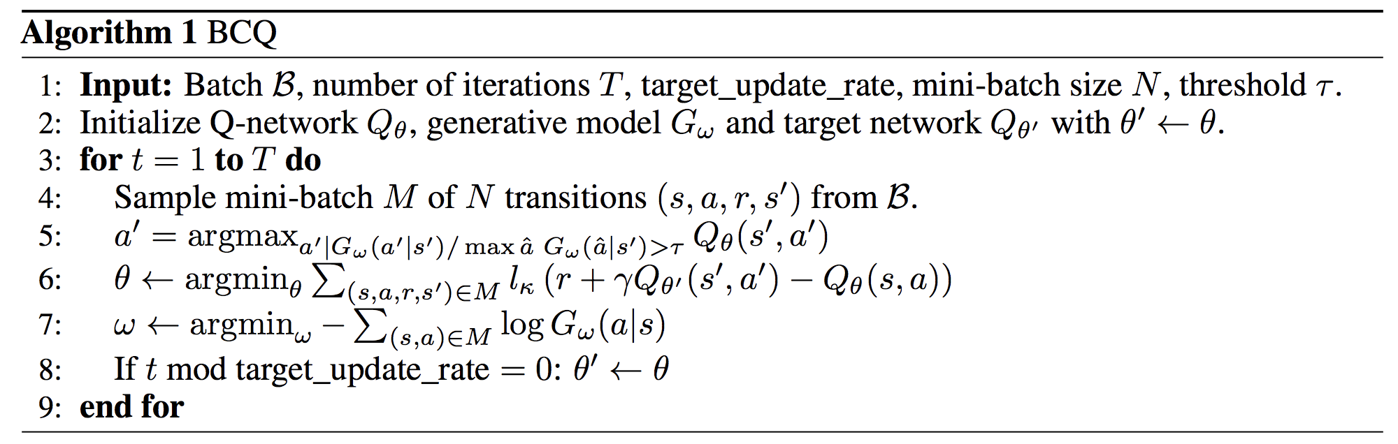
My “TL;DR”: train a behavior cloning network to predict actions of the behavior policy based on its states. For the Q-function update on iteration $k$, change the maximization over the successor state actions to only consider actions satisfying a threshold:
\[\mathcal{L}(\theta) = \ell_k \left(r + \gamma \cdot \Bigg( \max_{a' \; \mbox{s.t.} \; \frac{G_\omega(a'|s')}{\max \hat{a} \; G_\omega(\hat{a}|s')} > \tau} Q_{\theta'}(s',a') \Bigg) - Q_\theta(s,a) \right)\]When executing the policy during test-time rollouts, we can use a similar threshold:
\[\pi(s) = \operatorname*{argmax}_{a \; \mbox{s.t.} \; \frac{G_\omega(a'|s')}{\max \hat{a} \; G_\omega(\hat{a}|s')} > \tau} Q_\theta(s,a)\]Note the contrast where normally in Q-learning, we’d just do the max or argmax over the entire set of valid actions. Therefore, we will end up ignoring some actions that potentially have high Q-values, but that’s fine (and desirable!) if those actions have vastly over-estimated Q-values.
Some additional thoughts:
-
The parallels are obvious between $G_\omega$ in continuous versus discrete BCQ. In the continuous case, it is necessary to develop a generative model which may be complex to train. In the discrete case, it’s much simpler: run behavior cloning!
-
I was confused about why BCQ does the behavior cloning update of $\omega$ inside the for loop, rather than beforehand. Since the data is fixed, this seems suboptimal since the optimization for $\theta$ will rely on an inaccurate model $G_\omega$ during the first few iterations. After contacting Fujimoto, he agreed that it is probably better to move the optimization before the loop, but his results were not significantly better.
-
There is a $\tau$ parameter we can vary. What happens when $\tau = 0$? Then it’s simple: standard Q-learning, because any action should have non-zero probability from the generative model. Now, what about $\tau=1$? In practice, this is exactly behavior cloning, because when the policy selects actions it will only consider the action with highest $G_\omega$ value, regardless of its Q-value. The actual Q-learning portion of BCQ is therefore completely unnecessary since we ignore the Q-network!
-
According to the appendix, they use $\tau = 0.3$.
There are no theoretical results here; the paper is strictly experimental. The experiments are on nine Atari games. The batch of data is generated from a partially trained DQN agent over 10M steps (50M steps is standard). Note the critical design choice of whether:
- we take a single fixed snapshot (i.e., a stationary policy) and roll it out to get steps, or
- we take logged data from an agent during its training run (i.e., a non-stationary policy).
Fujimoto implements the first case, arguing that it is more realistic, but I think that claim is highly debatable. Since the policy is fixed, Fujimoto injects noise by setting $\epsilon=0.2$ 80% of the time, and setting $\epsilon=0.001$ otherwise. This must be done on a per-episode basis — it doesn’t make sense to change epsilons within an episode!
What are some conclusions from the paper?
-
Discrete BCQ seems to be the best of the “batch RL” algorithms tested. But the curves look really weird: BCQ performance shoots up to be at or slightly above the noise-free policy, but then stagnates! I should also add: exceeding the underlying noise-free policy is nice, but the caveat is that it’s from a partially trained DQN, which is a low bar.
-
For the “standard” off-policy algorithms of DQN, QR-DQN, and REM, QR-DQN is the winner, but still under-performs a noisy behavior policy, which is unsatisfactory. Regardless, trying QR-DQN in an offline setting, even though it’s not specialized for that case, might be a good idea if the dataset is large enough.
-
Results confirm some results from (Agarwal et al., 2020) in that distributional RL aids in exploitation), but that the success they were observing is highly specific to settings Agarwal used: a full 50M history of a teacher’s replay buffer, with a changing snapshot, plus noise from sticky actions.
Here’s a summary of results in their own words:
Although BCQ has the strongest performance, on most games it only matches the performance of the online DQN, which is the underlying noise-free behavioral policy. These results suggest BCQ achieves something closer to robust imitation, rather than true batch reinforcement learning when there is limited exploratory data.
This brings me to one of my questions (or aspirations, if you put it that way). Is it possible to run offline RL, and reliably exceed the noise-free behavior policy? That would be a dream scenario indeed.
Stabilizing Off-Policy Q-Learning via Bootstrapping Error Reduction
This NeurIPS 2019 paper is highly related to Fujimoto’s BCQ paper covered earlier, in that it also focuses on an algorithm to constrain the distribution of actions considered when running Q-learning in a pure off-policy fashion. It identifies a concept known as bootstrapping error which is clearly described in the abstract alone:
We identify bootstrapping error as a key source of instability in current methods. Bootstrapping error is due to bootstrapping from actions that lie outside of the training data distribution, and it accumulates via the Bellman backup operator. We theoretically analyze bootstrapping error, and demonstrate how carefully constraining action selection in the backup can mitigate it.
I immediately thought: what’s the difference between bootstrapping error here versus extrapolation error from (Fujimoto et al., 2019)? Both terms can be used to refer to the same problem of propagating inaccurate Q-values during Q-learning. However, extrapolation error is a broader problem that appears in supervised learning contexts, whereas bootstrapping is specific to reinforcement learning algorithms that rely on bootstrapped estimates.
The authors have an excellent BAIR Blog post which I highly recommend because it provides great intuition on how bootstrapping error affects offline Q-learning on static datasets. For example, this figure below shows that in the second plot, we may have actions $a$ that are outside the distribution of actions (OOD is short for out-of-distribution) induced by the behavior policy $\beta(a|s)$, indicated with the dashed line. Unfortunately, if those actions have $Q(s,a)$ values that are much higher, then they are used in the bootstrapping process for Q-learning to form the targets for Q-learning updates.

Incorrectly high Q-values for OOD actions may be used for backups, leading to
accumulation of error. Figure and caption credit: Aviral Kumar.
They also have results showing that if one runs a standard off-the-shelf off-policy (not offline) RL algorithm, that simply increasing the size of the static dataset does not appear to mitigate performance issues – which suggests the need for further study.
The main contributions of their paper are: (a) theoretical analysis that carefully constraining the actions considered during Q-learning can mitigate error propagation, and (b) a resulting practical algorithm known as “Bootstrapping Error Accumulation Reduction” (BEAR). (I am pretty sure that “BEAR” is meant to be a spin on “BAIR,” which is short for Berkeley Artificial Intelligence Research.)
The BEAR algorithm is visualized below. The intuition is to ensure that the learned policy matches the support of the action distribution from the static data. In contrast, an algorithm such as BCQ focuses on distribution matching (center). This distinction is actually pretty powerful; only requiring a support match is a much weaker assumption, which enables Offline RL to more flexibly consider a wider range of actions so long as the batch of data has used those actions at some point with non-negligible probability.

Illustration of support constraint (BEAR) (right) and distribution-matching
constraint (middle). Figure and caption credit: Aviral Kumar.
To enforce this in practice, BEAR uses what’s known as the Maximum Mean Discrepancy (MMD) distance between actions from the unknown behavior policy $\beta$ and the actor $\pi$. This can be estimated directly from samples. Putting everything together, their policy improvement step for actor-critic algorithms is succinctly represented by Equation 1 from the paper:
\[\pi_\phi := \max_{\pi \in \Delta_{|S|}} \mathbb{E}_{s \sim \mathcal{D}} \mathbb{E}_{a \sim \pi(\cdot|s)} \left[ \min_{j=1,\ldots,K} \hat{Q}_j(s, a)\right] \quad \mbox{s.t.} \quad \mathbb{E}_{s \sim \mathcal{D}} \Big[ \text{MMD}(\mathcal{D}(\cdot|s), \pi(\cdot|s)) \Big] \leq \varepsilon\]The notation is described in the paper, but just to clarify: $\mathcal{D}$ represents the static data of transitions collected by behavioral policy $\beta$, and the $j$ subscripts are from the ensemble of Q-functions used to compute a conservative estimate of Q-values. This is the less interesting aspect of the policy update as compared to the MMD constraint; in fact the BAIR Blog post doesn’t include the ensemble in the policy update. As far as I can tell, there is no ablation study that tests just using one or two Q-networks, so I wonder which of the two is more important: the ensemble of networks, or the MMD constraint?
The most closely related algorithm to BEAR is the previously-discussed BCQ (Fujimoto et al., 2019). How do they compare? The BEAR authors (Kumar et al., 2019) claim:
-
Their theory shows convergence properties under weaker assumptions, and they are able to bound the suboptimality of their approach.
-
BCQ is generally better when off-policy data is collected by an expert, but BEAR is better when data is collected by a weaker (or even random) policy. They claim this is because BCQ too aggressively constrains the distribution of actions, and this matches the interpretation of BCQ as matching the distribution of the policy of the data batch, whereas BEAR focuses on only matching the action support.
Upon reading this, I became curious to see if there’s a way to combine the strengths of both of the algorithms. I am also not entirely convinced that MuJoCo is the best way to evaluate these algorithms, so we should hopefully look at what other datasets might appear in the future so that we can perform more extensive comparisons of BEAR and BCQ.
At this point, we now consider papers that are in the second category – those which, rather than constrain actions in some way, focus on investigating what happens with a large and diverse dataset while maximizing the exploitation capacity of standard off-policy Deep RL algorithms.
An Optimistic Perspective on Offline Reinforcement Learning
Unlike the prior papers, which present algorithms to constrain the set of considered actions, this paper argues that it is not necessary to use a specialized Offline RL algorithm. Instead, use a stronger off-policy Deep RL algorithm with better exploitation capabilities. I especially enjoyed reading this paper, since it gave me insights on off-policy reinforcement learning, and the experiments are also clean and easy to understand. Surprisingly, it was rejected from ICLR 2020, and I’m a little concerned about how a paper with this many convincing experimental results can get rejected. The reviewers also asked why we should care about Offline RL, and the authors gave a rather convincing response! (Fortunately, the paper eventually found a home at ICML 2020.)
Here is a quick summary of the paper’s experiments and contributions. When discussing the paper or referring to figures, I am referencing the second version on arXiv, which corresponds to the ICLR 2020 submission and used “Batch RL” instead of “Offline RL” so we’ll use both terms interchangeably. The paper was previously titled “Striving for Simplicity in Off-Policy Deep Reinforcement Learning.”
-
To form the batch for Offline RL, they use logged data from 50M steps of standard online DQN training. In general, one step is four environment frames, so this matches the 200M frame case which is standard for Atari benchmarks. I believe the community has settled on the 1 step to 4 frame ratio. As discussed in (Machado et al., 2018), to introduce stochasticity, the agents employ sticky actions. So, given this logged data, let’s run Batch RL, where we run off-policy deep Q-learning algorithms with a 50M-sized replay buffer, and sample items uniformly.
-
They show that the off-policy, distributional-based DeepRL algorithms Categorical DQN (i.e., C51) and Quantile Regression DQN (i.e., QR-DQN), when trained solely on that logged data (i.e., in an offline setting), actually outperform online DQN!! See Figure 2 in the paper, for example. Be careful about what this claims means: C51 and QR-DQN are already known to be better than vanilla DQN, but the experiments show that even in the absence of exploration for those two methods, they still out-perform online (i.e., with exploration) DQN.
-
Incidentally, offline C51 and offline QR-DQN also out-perform offline DQN, which as expected, is usually worse than online DQN. (To be fair, Figure 2 suggests that in 10-15 out of 60 games, offline DQN can actually outperform the online variant.) Since the experiments disentangle exploration from exploitation, we can explain the difference between performance of offline DQN versus offline C51 or QR-DQN as due to exploitation capability.
-
Thus so far we have the following algorithms, from worst to best with respect to game score: offline DQN, online DQN, offline C51, and offline QR-DQN. They did not present a full result of offline C51 except for a few games in the Appendix but I’m assuming that QR-DQN would be better in both offline and online cases. In addition, I also assume that online C51 and online QR-DQN would outperform their offline variants, at least if their offline variants are trained on DQN-generated data.
-
To add further evidence that improving the base off-policy Deep RL algorithm can work well in the Batch RL setting, their results in Figure 4 suggest that using Adam as the optimizer instead of RMSprop for DQN is by itself enough to get performance gains. In that this offline DQN can even outperform online DQN on average! I’m not sure how much I can believe this result, because Adam can’t offer that much of an improvement, right?
-
They also experiment with a continuous control variant, using 1M samples from a logged training run of DDPG. They apply Batch-Constrained Q-learning from (Fujimoto et al., 2019) as discussed above, and find that it performs reasonably well. But they also find that they can simply use Twin-Delayed DDPG (i.e., TD3) from (Fujimoto et al., 2018) (yes, the same guy!) and train normally in an off-policy fashion to get better results than offline DDPG. Since TD3 is known as a stronger off-policy continuous control deep Q-learning algorithm than DDPG, this further bolsters the paper’s claims that all we need is a stronger off-policy algorithm for effective Batch RL.
-
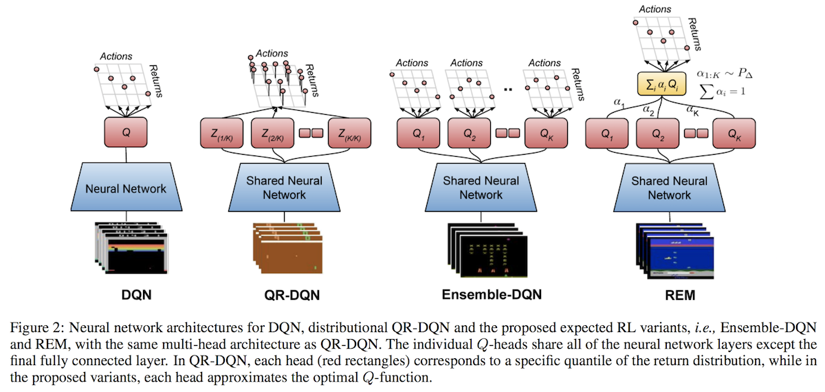
Finally, from the above observations, they propose their Random Ensemble Mixture (REM) algorithm, which uses an ensemble of Q-networks and enforces Bellman consistency among random convex combinations. This is similar to how Dropout works. There are offline and online versions of it. In the offline setting, REM outperforms C51 and QR-DQN despite being simpler. By “simpler” the authors mainly refer to not needing to estimate a full distribution of the value function for a given state, as distributional methods do.
That’s not all they did. In an older version of the paper, they also tried experiments with logged data from a training run of QR-DQN. However, the lead author told me he removed those results since there were too many experiments which were confusing readers. In addition, for logged data from training QR-DQN, it is necessary to train an even stronger off-policy Deep RL algorithm to out-perform the online QR-DQN algorithm. I have to admit, sometimes I was also losing track of all the experiments being run in this paper.
Here is a handy visualization of some algorithms involved in the paper: DQN, QR-DQN, Ensemble-DQN (their baseline) and REM (their algorithm):
My biggest takeaway from reading this paper is that in Offline RL, the quality of the data matters significantly, and it is better to use data from many different policies rather than one fixed policy. That they get logged data from a training run means that, literally, every four steps, there was a gradient update to the policy parameters and thus a change to the policy itself. This induces great diversity in the data for Offline RL. Indeed, (Fujimoto et al., 2019) argues that the success of REM and off-policy algorithms more generally depends on the training data composition. Thus, it is not generally correct to think of these papers contradicting each other; they are more accurately thought of as different ways to achieve the same goal. Perhaps the better way going forward is simply to use larger and larger datasets with strong off-policy algorithms, while also perhaps specializing those off-policy algorithms for the batch setting.
IRIS: Implicit Reinforcement without Interaction at Scale for Learning Control from Offline Robot Manipulation Data
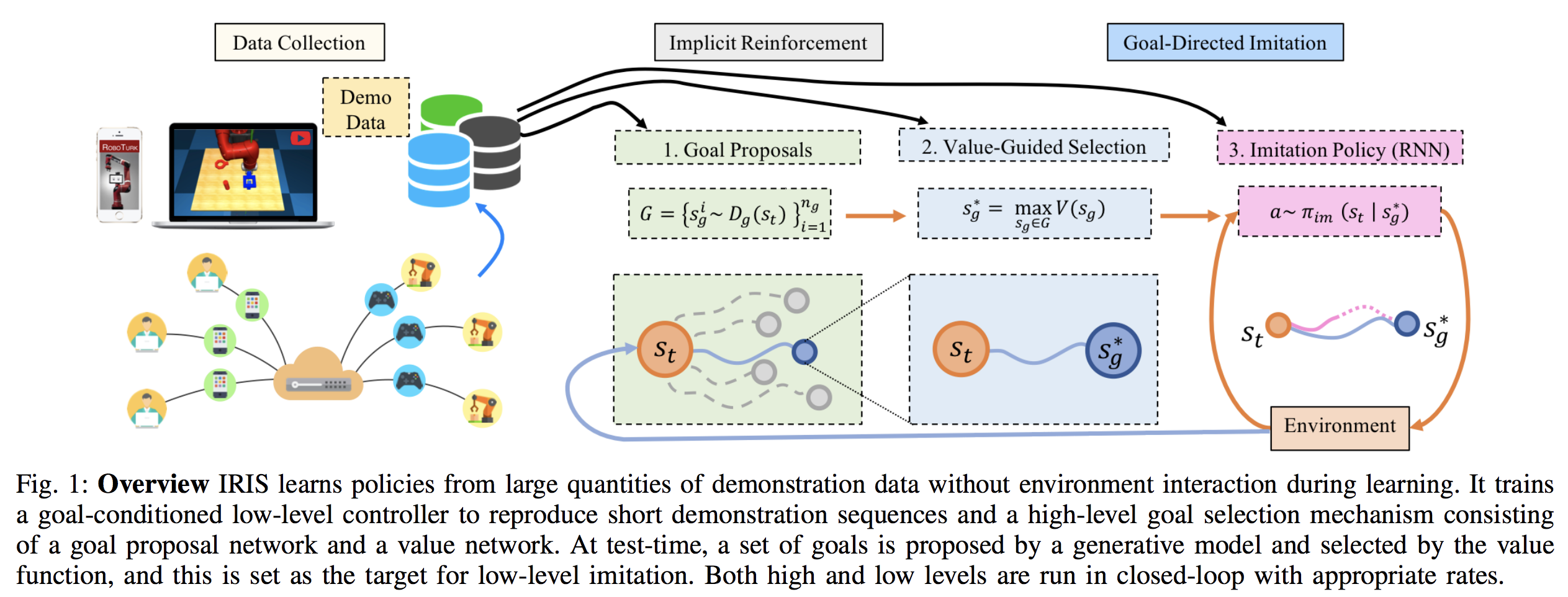
This paper proposes the algorithm IRIS: Implicit Reinforcement without Interaction at Scale. It is specialized for offline learning from large-scale robotics datasets, where the demonstrations may be either suboptimal or highly multi-modal. The algorithm is motivated by the same off-policy, Batch RL considerations as other papers I discuss here, and I found this paper because it cited a bunch of them. Their algorithm is visualized below:
To summarize:
-
IRIS splits control into “high-level” and “low-level” controllers. The high-level mechanism, at a given state $s_t$, must pick a new goal state $s_g$. Then, the low-level mechanism is conditioned on that goal state, and produces the actual actions $a \sim \pi_{im} (s_t | s_g)$ to take.
-
The high-level policy is split in two parts. The first samples several goal proposals. The second picks the best goal proposal to pass to the low-level controller.
-
The low-level controller, given the goal $s_g$, takes $T$ actions conditioned on that goal. Then, it returns control to the high level policy, which re-samples the goal state.
-
The episode terminates when the agent gets sufficiently close to the true goal state. This is a continuous state domain, so they simply pick a distance threshold to the state. They are also in the sparse reward domain, adding another challenge.
How are the components trained?
-
The first part of the high-level controller uses a goal conditional Variational AutoEncoder (cVAE). Given a sequence of states in the data, IRIS samples pairs that are $T$ time steps apart, i.e., $(s_t, s_{t+T})$. The encoder $E(s_{t},s_{t+T})$ maps the tuple to a set of latent variables for a Gaussian, i.e., $\mu, \sigma =E(s_{t},s_{t+T})$. The decoder must construct the future state: $\hat{s}_{t+T} \sim D(s_t, z)$ where $z$ is a Gaussian sampled from $\mu$ and $\sigma$. This is for training; for test time, they sample $z$ from a standard normal $z \sim \mathcal{N}(0,1)$ (with regularization during training) and pass it to the decoder, so that it produces goal states.
-
The second part uses an action cVAE as part of their simpler variant of Batch Constrained Deep Q-learning (discussed at the beginning of this blog post) for the value function in the high-level controller. This cVAE, rather than predicting goals, will predict actions conditioned on a state. This can be trained by sampling state-action pairs $(s_t,a_t)$ and having the cVAE predict $a_t$. They can then use it in their BCQ algorithm because the cVAE will model actions that are more likely to be part of the training data.
-
The low-level controller is a recurrent neural network that, given $s_t$ and $s_g$, produces $a_t$. It is trained with behavior cloning, and therefore does not use Batch RL. But, how does one get the goal? It’s simple: since IRIS assumes the low-level controller runs for a fixed number of steps (i.e., $T$ steps) then they take consecutive state-action sequences of length $T$ and then treat the last state as the goal. Intuitively, the low-level controller trained this way will be able to figure out how to get from a start state to a “goal” state in $T$ steps, where “goal” is in quotes because it is not a true environment goal but one which we artificially set for training. This reminds me of Hindsight Experience Replay, which I have previously dissected.
Some other considerations:
-
They argue that IRIS is able to handle diverse solutions because the goal cVAE can sample different goals, to explicitly take diversity into account. Meanwhile, the low-level controller only has to model short-horizon goals at a time “resolution” that does not easily permit many solutions.
-
They argue that IRIS can handle off-policy data because their BCQ will limit actions to those likely to be generated by the data, and hence the value function (which is used to select the goal) will be more accurate.
-
They split IRIS into higher and lower level controllers because in theory this may help to handle for suboptimal demonstrations — the high-level controller can pick high value goals, and the low-level controller just has to get from point A to point B. This is also pretty much why people like hierarchies in general.
Their use of Batch RL is interesting. Rather than using it to train a policy, they are only using it to train a value function. Thus, this application can be viewed as similar to papers that are concerned with off-policy RL but only for the purpose of evaluating states. Also, why do they argue their variant of BCQ is simpler? I think it is because they eschew from training a perturbation model, which was used to optimally perturb the actions that are used for candidates. They also don’t seem to use a twin critic.
They evaluate IRIS on three datasets. Two use their prior work, RoboTurk. You can see an overview on the Stanford AI Blog here. I have not used RoboTurk before so it may be hard for me to interpret their results.
-
Graph Reach: they use a simple 2D navigation example, which is somewhat artificial but allows for easy testing of multi-modal and suboptimal examples. Navigation tasks are also present in other papers that test for suboptimal demonstrations, such as SAVED from Ken Goldberg’s lab.
-
Robosuite Lift: this involves the Robosuite Lift data, where a single human performed teleoperation (in simulation) using RoboTurk, to lift an object. The human intentionally used suboptiomal demonstrations..
-
RoboTurk Can Pick and Place: now they use a pick-and-place task, this time using RoboTurk to get a diverse set of samples due to using different human operators. You can see an overview on the Stanford AI Blog here. Again, I have not used Roboturk, but it appears that this is the most “natural” of the environments tested.
Their experiments benchmark against BCQ, which is a reasonable baseline.
Overall, I think this paper has a mix of both the “action constraining” algorithms discussed in this blog post, and the “learning from large scale datasets” papers. It was the first to show that offline RL could be used as part of the process for robot manipulation. Another project that did something similar, this time with physical robots, is from DeepMind, to which we now turn.
Scaling Data-driven Robotics with Reward Sketching and Batch Reinforcement Learning
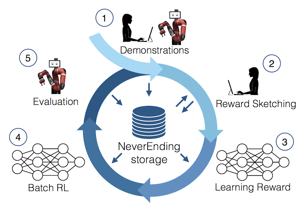
This recent DeepMind paper is the third one I discuss which highlights the benefits of a large, massive offline dataset (which they call “NeverEnding Storage”) coupled with a strong off-policy reinforcement learning algorithm. It shows what is possible when combining ideas from reinforcement learning, human-computer interaction, and database systems. The approach consists of five major steps, as nicely indicated by the figure:
In more detail, they are:
-
Get demonstrations. This can be from a variety of sources: human teleoperation, scripted policies, or trained policies. At first, the data is from human demonstrations or scripted policies. But, as robots continue to train and perform tasks, their own trajectories are added to the NeverEnding Storage. Incidentally, this paper considers the multi-task setup, so the policies act on a variety of tasks, each of which has its own starting conditions, particular reward, etc.
-
Reward sketching. A subset of the data points are selected for humans to indicate rewards. Since it involves human intervention, and because reward design is fiendishly difficult, this part must be done with care, and certainly cannot be done by having humans slowly and manually assign a number to every frame. (I nearly vomit when simply thinking about doing that.) The authors cleverly engineered a GUI where a human can literally sketch a reward, hence the name reward sketching, to seamlessly get rewards (between 0 and 1) for each frame.
-
Learning the reward. The system trains a reward function neural network $r_\psi$ to predict task-specific (dense) rewards from frames (i.e., images). Rather than regress directly on the sketched values, the proposed approach involves taking two frames $x_t$ and $x_q$ within the same episode, and enforcing consistency conditions with the reward functions via hinge losses. Clever! When the reward function updates, this can trigger retroactive re-labeling of rewards per time step in the NES.
-
Batch RL. A specialized Batch RL algorithm is not necessary because of the massive diversity of the offline dataset, though they do seem to train task-specific policies. They use a version of D4PG, short for “Distributed Distributional Deep Deterministic Policy Gradients” which is … a really good off-policy RL algorithm! Since the NES contains data from many tasks, if they are trying to optimize the learned reward for a task, they will draw 75% of the minibatch from all of the NES, and draw the remaining 25% from task-specific episodes. I instantly made the connection to DeepMind’s “Observe and Look Further (arXiv 2018)” paper (see my blog post here) which implements a 75-25 minibatch ratio among demonstrator and agent samples.
-
Evaluation. Periodically evaluate the robot and add new demonstrations to NES. Their experiments consist of a Sawyer robot facing a 35 x 35 cm basket of objects, and the tasks generally involve grasping objects or stacking blocks.
-
Go back to step (1) and repeat, resulting in over 400 hours of video data.
There is human-in-the-loop involved, but they argue (reasonably, I would add) that reward sketching is a relatively simple way of incorporating humans. Furthermore, while human demonstrations are necessary, those are ideally drawn from existing datasets.
They say they will release their dataset so that it can facilitate development of subsequent Batch RL algorithms, though my impression is that we might as well deploy D4PG, so I am not sure if this will spur more Batch RL algorithms. On a related note, if you are like me and have trouble following all of the “D”s in the algorithm and all of DeepMind’s “state of the art” reinforcement learning algorithms, DeepMind has a March 31 blog post summarizing the progression of algorithms on Atari. I wish we had something similar for continuous control, though.
Here are some comparisons between this and the ones from (Agarwal et al., 2020) and (Mandlekar et al., 2020) previously discussed:
-
All papers deal with Batch RL from a large set of robotics-related data, though the datasets themselves differ: Atari versus RoboTurk versus this new dataset, which will hopefully be publicly available. This paper appears to be the only one capable of training Batch RL policies to perform well on new tasks. The analogue for Atari would be training a Batch RL agent on several games, and then applying it (or fine-tuning it) to a new Atari game, but I don’t think this has been done.
-
This paper agrees with the conclusions of (Agarwal et al., 2020) that having a sufficiently large and diverse dataset is critical to the success of Offline RL.
-
This paper uses D4PG as a very powerful, offline RL algorithm for learning policies, whereas (Agarwal et al., 2020) proposes a simpler version of Quantile-Regression DQN for discrete control, and (Mandlekar et al., 2020) only use Batch RL to train a value function instead of a policy.
-
This paper proposes the novel reward sketching idea, whereas (Agarwal et al., 2020) only use environments that give dense rewards, and (Mandlekar et al., 2020) use environments with sparse rewards that indicate task success.
-
This paper does not factorize policies into lower and higher level controllers, unlike (Mandkelar et al., 2020), though I assume in principle it is possible to merge the ideas.
In addition to the above comparisons, I am curious about the relationship between this paper and RoboNet from CoRL 2019. It seems like both projects are motivated by developing large datasets for robotics research, though the latter may be more specialized to visual foresight methods, but take my judgment with a grain of salt.
Overall, I have hope that, with disk space getting cheaper and cheaper, we will eventually have robots deployed in fleets that can draw upon this storage in some way.
Concluding Remarks and References
What are some of the common themes or thoughts I had when reading these and related papers? Here are a few:
-
When reading these papers, take careful note as to whether the data is generated from a non-stationary or a stationary policy. Furthermore, how diverse is the dataset?
-
The “data diversity” and “action constraining” aspects of this literature may be complementary, but I am not sure if anyone has shown how well those two mix.
-
As I mention in my blog posts, it is essential to figure out ways that an imitator can outperform the expert. While this has been demonstrated with algorithms that combine RL and IL with exploration, the Offline RL setting imposes extra constraints. If RL is indeed powerful enough, maybe it is still able to outperform the demonstrator in this setting. Thus, when developing algorithms for Offline RL, merely meeting the demonstrator behavior is not sufficient.
Happy offline reinforcement learning!
Here is a full listing of the papers covered in this blog post, in order of when I introduced the paper.
-
Sascha Lange, Thomas Gabel, Martin Riedmiller. Batch Reinforcement Learning. Book Chapter, “Reinforcement Learning: State of the Art,” 2012.
-
Sergey Levine, Aviral Kumar, George Tucker, Justin Fu. Offline Reinforcement Learning: Tutorial, Review, and Perspectives on Open Problems, arXiv 2020.
-
Scott Fujimoto, David Meger, Doina Precup. Off-Policy Deep Reinforcement Learning without Exploration, ICML 2019.
-
Scott Fujimoto, Edoardo Conti, Mohammad Ghavamzadeh, Joelle Pineau. Benchmarking Batch Deep Reinforcement Learning Algorithms, NeurIPS 2019 workshop.
-
Aviral Kumar, Justin Fu, George Tucker, Sergey Levine. Stabilizing Off-Policy Q-Learning via Bootstrapping Error Reduction, NeurIPS 2019.
-
Rishabh Agarwal, Dale Schuurmans, Mohammad Norouzi. An Optimistic Perspective on Offline Reinforcement Learning, ICML 2020.
-
Ajay Mandlekar, Fabio Ramos, Byron Boots, Silvio Savarese, Li Fei-Fei, Animesh Garg, Dieter Fox. IRIS: Implicit Reinforcement without Interaction at Scale for Learning Control from Offline Robot Manipulation Data, ICRA 2020.
-
Serkan Cabi, Sergio Gómez Colmenarejo, Alexander Novikov, Ksenia Konyushkova, Scott Reed, Rae Jeong, Konrad Zolna, Yusuf Aytar, David Budden, Mel Vecerik, Oleg Sushkov, David Barker, Jonathan Scholz, Misha Denil, Nando de Freitas, Ziyu Wang. Scaling Data-driven Robotics with Reward Sketching and Batch Reinforcement Learning, RSS 2020.
Finally, here are another set of Offline RL or related references that I didn’t have time to cover, but I will likely modify this post in the future, especially given that I already have summary notes to myself on most of these papers (but they are not yet polished enough to post on this blog).
-
Romain Laroche, Paul Trichelair, Rémi Tachet des Combes. Safe Policy Improvement with Baseline Bootstrapping, ICML 2019.
-
Natasha Jaques, Asma Ghandeharioun, Judy Hanwen Shen, Craig Ferguson, Agata Lapedriza, Noah Jones, Shixiang Gu, Rosalind Picard. Way Off-Policy Batch Deep Reinforcement Learning of Human Preferences in Dialog, arXiv 2019.
-
Xinyue Chen, Zijian Zhou, Zheng Wang, Che Wang, Yanqiu Wu, Keith Ross. BAIL: Best-Action Imitation Learning for Batch Deep Reinforcement Learning, arXiv 2019.
-
Yifan Wu, George Tucker, Ofir Nachum. Behavior Regularized Offline Reinforcement Learning, arXiv 2019.
-
Noah Y. Siegel, Jost Tobias Springenberg, Felix Berkenkamp, Abbas Abdolmaleki, Michael Neunert, Thomas Lampe, Roland Hafner, Nicolas Heess, Martin Riedmiller. Keep Doing what Worked: Behavior Modelling Priors for Offline Reinforcement Learning, ICLR 2020.
-
Justin Fu, Aviral Kumar, Ofir Nachum, George Tucker, Sergey Levine. D4RL: Datasets for Deep Data-Driven Reinforcement Learning. arXiv 2020.
-
Aviral Kumar, Abhishek Gupta, Sergey Levine. DisCor: Corrective Feedback in Reinforcement Learning via Distribution Correction, arXiv 2020.
-
Aviral Kumar, Aurick Zhou, George Tucker, Sergey Levine. Conservative Q-Learning for Offline Reinforcement Learning, arXiv 2020.
-
Ashvin Nair, Murtaza Dalal, Abhishek Gupta, Sergey Levine. Accelerating Online Reinforcement Learning with Offline Datasets, arXiv 2020.
-
Tatsuya Matsushima, Hiroki Furuta, Yutaka Matsuo, Ofir Nachum, Shixiang Gu. Deployment-Efficient Reinforcement Learning via Model-Based Offline Optimization, arXiv 2020.
-
Rahul Kidambi, Aravind Rajeswaran, Praneeth Netrapalli, Thorsten Joachims. MOReL: Model-Based Offline Reinforcement Learning, arXiv 2020.
-
Tianhe Yu, Garrett Thomas, Lantao Yu, Stefano Ermon, James Zou, Sergey Levine, Chelsea Finn, Tengyu Ma. MOPO: Model-based Offline Policy Optimization, arXiv 2020.
-
Ziyu Wang, Alexander Novikov, Konrad Żołna, Jost Tobias Springenberg, Scott Reed, Bobak Shahriari, Noah Siegel, Josh Merel, Caglar Gulcehre, Nicolas Heess, Nando de Freitas. Critic Regularized Regression, arXiv 2020.
There is also extensive literature on off-policy evaluation, without necessarily focusing on policy optimization or deploying learned policies in practice. I did not focus on these as much since I wanted to discuss work that trains policies in this post.
I hope this post was helpful! As always, thank you for reading.