Read-Through of Multi-Level Discovery of Deep Options

In this post, I attempt to learn as much as possible about the paper Multi-Level Discovery of Deep Options, which introduced the DDO algorithm. This post is split into my understanding of the math, followed by implementation/experiments.

Before we begin, here is some useful notation:

• Options are denoted as \(h = \langle \pi_h, \psi_h \rangle \in \mathcal{H}\), with \(\mathcal{H}\) representing the set of possible options. To make the notation clearer when we’re dealing with options at each time step \(t\), we could write \(\mathcal{H} = \{h_{\rm opt}^{(1)}, \ldots, h_{\rm opt}^{|\mathcal{H}|}\}\).

• Higher-level policies are denoted as \(\eta(h \mid s)\), in which we pick options. You could also repeat this recursively; think of using something like \(\eta'(\eta \mid s)\), though the paper never officially uses that notation.

• A set of \(K\) demonstrations are denoted as \(\{\xi_1, \ldots, \xi_K\}\). They do not assume that these demonstrations are from an expert supervisor, only that (a) they have some hierarchical structure to be discovered, and (b) that they are informative of the relevant actions to take in each state. Assumption (a) is easier to understand and justify, for if we didn’t have a hierarchical structure to discover, there is no point doing DDO or any hierarchical learning algorithm. Fortunately, in many real-life tasks (for humans), we have hierarchical structures.

The paper also goes through some usual reinforcement learning and imitation learning notation, which I won’t repeat here as it will be clear to those with the relevant background.

The goal of DDO is to discover a set of parameterized options from \(\{\xi_1, \ldots, \xi_K\}\).

The Math

To derive the math, the authors use the perspective of fitting a generative model to the trajectories. That generative model, however, has latent variables, so they need to perform a flavor of Expectation-Maximization, which I’ve previously blogged about here.

But what are the latent (a.k.a., hidden) variables?

• The choice of \(h_t \in \mathcal{H}\), which represents the option at time \(t\).

• In addition, their generative model also assumes that at each time step, we have a binary random variable \(b_t \in \{ 0, 1 \}\), where if \(b_t=1\), a new option is drawn from the high-level policy. The random variable follows a Bernoulli distribution with parameter based on the option termination conditions \(\psi_h\); the higher the value at a given state, the more likely it is that the option should finish and return control to the meta-policy.

The generative model tells us how to assign probabilities to the trajectories. Now, let’s figure out how to find \(\theta \in \Theta\) that maximizes the likelihood of the trajectories! We’re using \(\theta\) to denote all the parameters of everything together: the meta-control policy and for each option. The derivation here assumes a two-level hierarchy, but the extension to multiple levels should be straightforward, besides some nightmarish notation.

The discussion above makes it clear that the \(i\)th trajectory in our data follows this structure:

with \(\xi_i\) and \(\zeta_i\) representing the visible and latent variables, respectively.

To find parameters, we need to encode this probabilistically, as in \(p(\xi_i, \zeta_i)\). Fortunately, as is standard in RL/IL, this long joint probability decomposes based on time steps. Specifically, we express it as:

where for notational clarity, we denote the various probability distributions as follows:

• \(p_0\) represents the probability distribution over the initial state. There is no dependence on \(\theta\).
• \(p(s' | s,a)\) represents the dynamics of the environment. Once again, there is no dependence on \(\theta\).
• \(q_\theta(b_t,h_t | h_{t-1},s_t)\) represents the distribution over the hidden variables. (My notation is slightly different than what the DDO paper uses, but I find it easier to think of the entire likelihood \(\mathbb{P}_\theta\) as distinct from this.)
• \(\pi\) and \(\eta\), of course, represent the policy and option selection.

Since \(b\) is Bernoulli, we can easily split \(q_\theta\) into cases to define it more precisely:

and

We should now step back and ask ourselves if this definition of \(\mathbb{P}_\theta(\zeta_i, \xi_i)\) makes sense. Does it?

Yes. The first few terms draw the initial state, and then the \(\delta_{b_0=1}\) ensures that we actually have an option to sample from to start (though it is really unnecessary notation). Then we assume we draw \(h_0\).

Next, we iterate through the remaining time steps. We draw the action based on the policy, and then the dynamics provide the state. But then we also need to sample the two latent variables. We’re packing these together in \(q_\theta\), but you can also think of it sequentially: first sampling a Bernoulli for the option termination, and then sampling from the meta-policy. The split of \(q_\theta\) in two cases makes the sequential aspect of this clearer: \(\psi_{h_{t-1}}\) represents the probability that \(b_t=1\), and if it is zero (with probability \(1-\psi_{h_{t-1}}\)), we don’t need to draw at all, hence the delta term \(\delta_{h_t=h_{t-1}}\). Otherwise, we need to sample, hence the \(\eta(h_t|s_t)\). Yes, this all makes sense, and can be reasoned by iterating through the generative model “pseudocode.”

Great. Now we know the likelihood of one trajectory. We want to maximize the (log) likelihood \(L(\theta | \xi)\) assigned to a trajectory, which means we need to take gradient steps to get our neural network weights to go to the correct spot. For one trajectory \(\xi\) (omitting the subscript which normally indicates which trajectory in our set of them), we have:

Where in (i) we substituted the definition with the thing we want to optimize since that will lead to “likely” trajectories learned from gradient steps, in (ii) we applied the \(\nabla \log p(x) = \frac{\nabla p(x)}{p(x)}\) “trick” and then applied the probability 101 rule that \(p(x) = \sum_z p(x,z)\) while explicitly writing out what it means to sum over the discrete-valued \(\zeta\) latent variable over all \(T\) times (this is an exponentially large sum!), in (iii) we again applied the same log-derivative trick, except this time from the perspective of \(\nabla p(x) = p(x) \nabla \log p(x)\), in (iv) we used the definition of conditional probability and then the definition of expectation in (v), and finally in (vi) we applied our previous derivation of the probability of both the visible and latent variables, and omitted terms which cancel out from the gradient. Recall again that \(\theta\) includes the parameters of the meta policy (i.e., \(\eta\)) and the lower-level options \(h_t \in \mathcal{H}\).

In general, we’re dealing with a batch of trajectories, so just apply it to each of the trajectories and take an average over the minibatch to make the gradient independent of batch size.

This is good, but we can actually write the gradient more explicitly, without the expectation by converting the expectation to the sums. Effectively, instead of doing the step (vi) to (v) thing we did earlier, we’ll explicitly simplify the probability based on the summation. However, we’ll start from step (vi) above since it’s easier to manage the calculations with all the stuff canceled out after applying \(\nabla_\theta\). We’ll go through this computation in several steps.

For the third term, we have:

Where (i) is by linearity of expectation, (ii) simplifies the expectation by realizing that the term under expectation only (directly) depends on \(h_t\), and (iii) applies the definition of expectation. If step (ii) isn’t clear, it should work out if you expand the full probability into sums over all \(h_t\) and all \(b_t\). Then the \(b_t\) sums should get “pushed to the right” and sum to one (and thus go away) and the rest should follow from there. I would write it out, except that it makes sense to me and I don’t want to spend my entire blogging career getting bogged down with notation.

Additional comment: it might also be the case that conditioning on \(\xi\) instead of just the relevant part of \(\xi\) was done for notational convenience.

Next, here’s how to rewrite the first two terms in the expectation. This requires a considerable amount of care:

For the most part, it uses similar techniques as the other part, such as converting the expectation to sums over probabilities (i.e., applying the definition) and then moving the sums to the right as far as possible so that they can sum to one and then eliminate. The main challenge here is tracking all the \(b_t\)s here in addition to the \(h_t\)s.

Putting all this together, we get the equation shown in the DDO paper where they’ve substituted in \(u_t(h), v_t(h)\), and \(w_t(h)\) terms. It should be equivalent to what I have above, though the odds that there is a typo somewhere (probably above) is 100 percent. I think I know how this works in theory but there is a lot of notation.

Incidentally, there is some good explanation about how — since we’re living in discrete-land — there are three cross entropy loss terms embedded into the gradient update.

The last piece of math to note before proceeding to the implementation details is … how to implement Expectation-Gradient efficiently. Fortunately, the Expectation step — where latent variables are “sampled” and weighted probabilistically — can be done with the Baum-Welch update, which I have previously blogged about. I won’t go through the details here, though I went through them on pencil and paper and the math makes sense. The key to my intuition is to think of forward and backward probabilities as “counting up” the number of ways to reach a given spot from the start (for trajectory prefixes) or the end (for trajectory suffixes). The Baum-Welch algorithm gives us efficient ways to compute various probabilities, and then, since we can formulate a loss function which is the negative log likelihood of a trajectory, we can call TensorFlow to compute gradients for us for the Gradient step. Thus, we have the Expectation-Gradient algorithm.

Quick note: recall Expectation-Maximization. They’re not doing that because the maximization part can’t be done in closed form with neural network models:

Our work is most related to [43], who use a similar generative model, originally introduced by [8] as an Abstract Hidden Markov Model, and learn its parameters via the Expectation-Maximization (EM) algorithm. EM applies the same forward-backward E-step as our Expectation-Gradient algorithm (Section 4.2) to compute marginal posteriors, but uses them for a complete optimization M-step over the options and the meta-control policies. This optimization is infeasible for expressive representations, as well as for multi-level hierarchies.

OK, now let’s move on to some of the implementation details and experimental results.

Implementation Details and Experiments

I am mostly going to investigate their GridWorld-related experiments, as the Atari stuff uses RAM, not images, so it’s hard to interpret, and the surgical robotics part is impossible to comprehend without intimate knowledge of the training data.

They consider DDO under two different scenarios:

(Supervised) given a supervisor who demonstrates a few times how to perform a task, show that the discovered options are useful for accelerating reinforcement learning on the same task; (Exploration) apply reinforcement learning for \(T\) episodes, sample trajectories from the current best policy, and augment the action space with the discovered options for the remaining \(T'\) episodes

This is a bit confusing to me for a few reasons. I will state why later when I review some questions I have about the paper. Let’s move on to GridWorld. Details:

• a \(15 \times 11\) grid, with four rooms.
• the agent actions is randomized with probability 0.3.
• the agent can move in four directions (the “atomic actions”), and moving into wall has no effect.
• an apple is spawned in random location, and upon reaching it the agent gets +1 reward (and then it is respawned).
• the agent knows where it is, as it’s hard-coded in the state space.

All neural network policies (for control, meta-control, termination) are neural nets with one hidden layer of … two nodes. Yeah, you don’t need much for GridWorld.

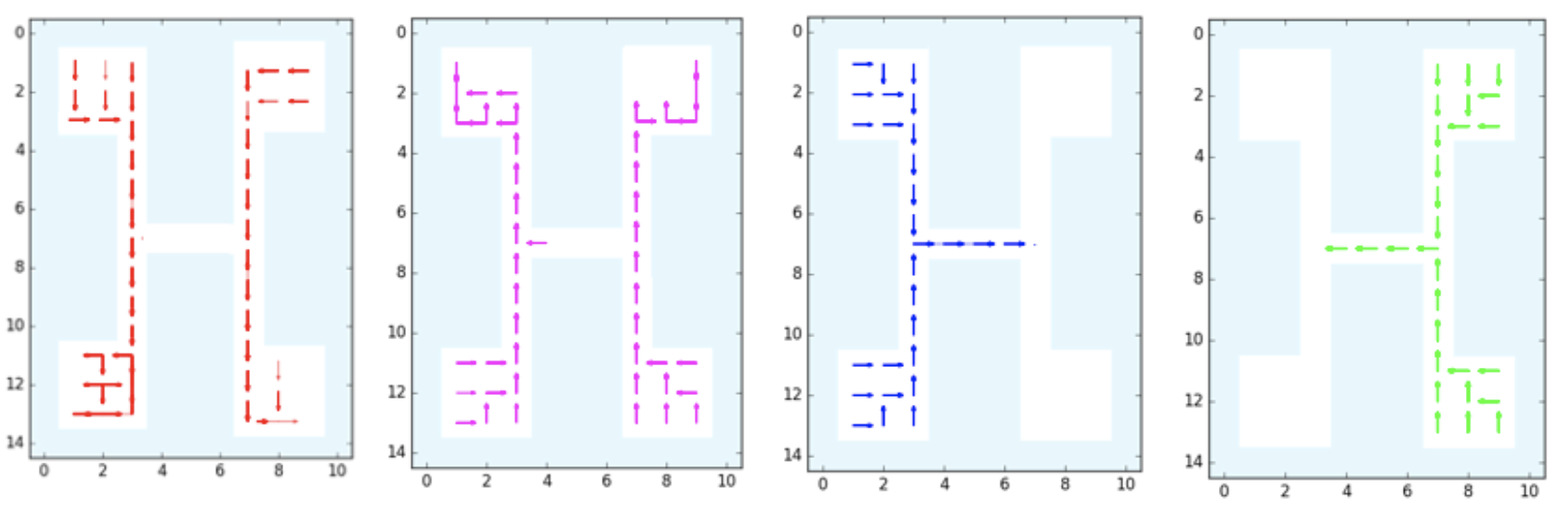The GridWorld used in the DDO paper. It is repeated four times in this image, each with a different discovered option: down, up, right, and left, respectively.

For the two setups:

• Supervised. They generate 50 trajectories of length 1000 using Value Iteration. (1000 seems like a large number, but the agent repeatedly respawns after hitting the apple so trajectories can go on indefinitely.) Then, after running DDO on this data, they can discover options. This is the supervised case, so there is (I assume) no environment interaction during the DDO stage. They executed the learned options and found four of them at the lower level (see figure above). There’s another figure for the higher-level options, which shows the options that are invoked to move the agents to rooms, starting from any given state.

• Exploration. They trained a DQN agent for 2000 steps with atomic actions. Then after those steps, they can roll out trajectories from the \(\epsilon\)-greedy policy, which effectively turn this into a “supervised” case. DDO learns options, and then the Q-function is then reset and DQN is run again with the augmented action space. I think what they want to show is that, compared to baseline DQN, the DQN augmented with options learns faster. It is a little hard to interpret Figure 2, though. They are starting from 2000 steps when they compute the number of steps for the option-augmented agents, right? (Because that’s 2000 steps of computation needed.) I think so, as their Figure 2 plots for the “exploration setting” are like the ones from the “supervised” setting except shifted to the right past 2000 steps, but then I’m surprised at why rewards shoot up at (essentially) exactly 2000 steps.

I also read through their Supplementary Material, which provides mostly more information on various GridWorld settings. Figure 7 appears to be missing the benchmark of having options-only DQN, but otherwise it has primitives-only DQN and options-and-primitives DQN, which is the “augmented DQN” from the paper.

Now here are some questions I have:

• For the supervised setting of DDO, is it fair to say it “accelerates RL”? In the default RL setting, we do not start with expert trajectories. Thus, any time we can get expert trajectories to bootstrap our starting policy, isn’t that an unfair advantage? This is what I wondered about when digesting the first half of Figure 2. Perhaps the comparison should be with reinforcement learning initialized with behavior cloning?

• For the exploration setting of DDO, what does it mean to augment the action space with discovered options? I think it means this: suppose our default action space is \(\mathcal{A} = \{a_1,a_2,a_3,a_4\}\). Then we discover three options, so the action space becomes \(\mathcal{A}' = \mathcal{A} \cup \{h_{\rm opt}^{(1)}, h_{\rm opt}^{(2)}, h_{\rm opt}^{(3)}\}\). Is that right? Then how is this logic implemented? The original RL policy must have started with a neural network that outputs four components, one per action (so that we can do a softmax to get the full probability distribution). Do we then copy weights over to a new neural network with seven outputs, so that all weights except for the last layer are pre-initialized?

• Regarding the DQN results, DQN is notorious for requiring lots of hyperparameter tuning and there are many ways that the implementation can go wrong. I wonder if this was hand-implemented or if the authors based it on an existing library with known benchmarks.

Whew! That was a fairly exhausting read. I needed to read this three times (which is the amount Professor Michael I. Jordan keeps telling us to read textbooks) but at least I think I get the gist of how DDO works.