Zero-Shot Visual Imitation
In this post, I will further investigate one of the papers I discussed in an earlier blog post: Zero-Shot Visual Imitation (Pathak et al., 2018).
For notation, I denote states and actions at some time step \(t\) as \(s_t\) and \(a_t\), respectively, if they were obtained through the agent exploring in the environment. A hat symbol, \(\hat{s}_t\) or \(\hat{a}_t\), refers to a prediction made from some machine learning model.
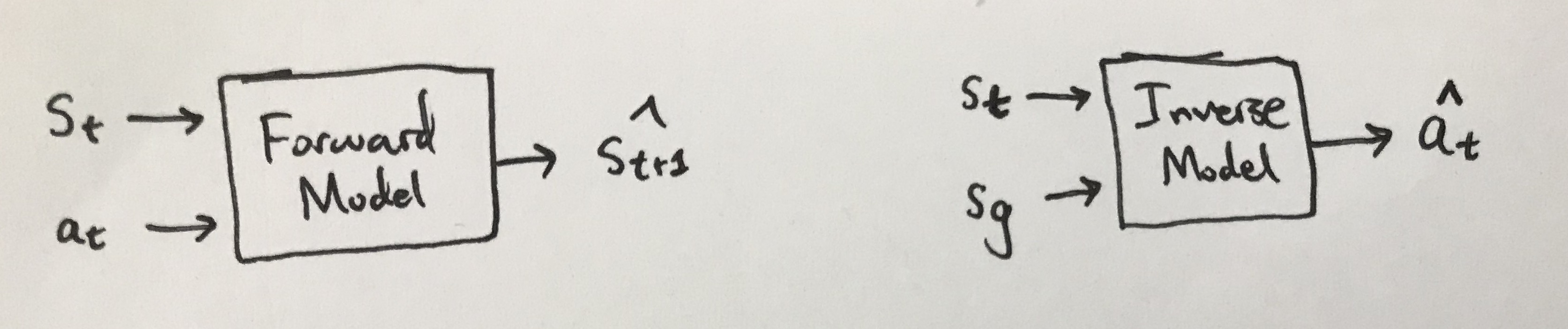
Basic forward (left) and inverse (right) model designs.
Recall the basic forward and inverse model structure (figure above). A forward model takes in a state-action pair and predicts the subsequent state \(\hat{s}_{t+1}\). An inverse model takes in a current state \(s_t\) and some goal state \(s_g\), and must predict the action that will enable the agent go from \(s_t\) to \(s_t\).
-
It’s easiest to view the goal input to the inverse model as either the very next state \(s_{t+1}\), or the final desired goal of the trajectory, but some papers also use \(s_g\) as an arbitrary checkpoint (Agrawal et al., 2016, Nair et al., 2017, Pathak et al., 2018). For the simplest model, it probably makes most sense to have \(s_g = s_{t+1}\) but I will use \(s_g\) to maintain generality. It’s true that \(s_g\) may be “far” from \(s_t\), but the inverse model can predict a sequence of actions if needed.
-
If the states are images, these models tend to use convolutions to get a lower dimensional featurized state representation. For instance, inverse models often process the two input images through tied (i.e., shared) convolutional weights to obtain \(\phi(s_t)\) and \(\phi(s_{t+1})\), upon which they’re concatenated and then processed through some fully connected layers.
As I discussed earlier, there are a number of issues related to this basic forward/inverse model design, most notably about (a) the high dimensionality of the states, and (b) the multi-modality of the action space. To be clear on (b), there may be many (or no) action(s) that let the agent go from \(s_t\) to \(s_g\), and the number of possibilities increases with a longer time horizon, if \(s_g\) is many states in the future.
Let’s understand how the model proposed in Zero-Shot Visual Imitation mitigates (b). Their inverse model takes in \(s_g\) as an arbitrary checkpoint/goal state and must output a sequence of actions that allows the agent to arrive at \(s_g\). To simplify the discussion, let’s suppose we’re only interested in predicting one step in the future, so \(s_g = s_{t+1}\). Their predictive physics design is shown below.
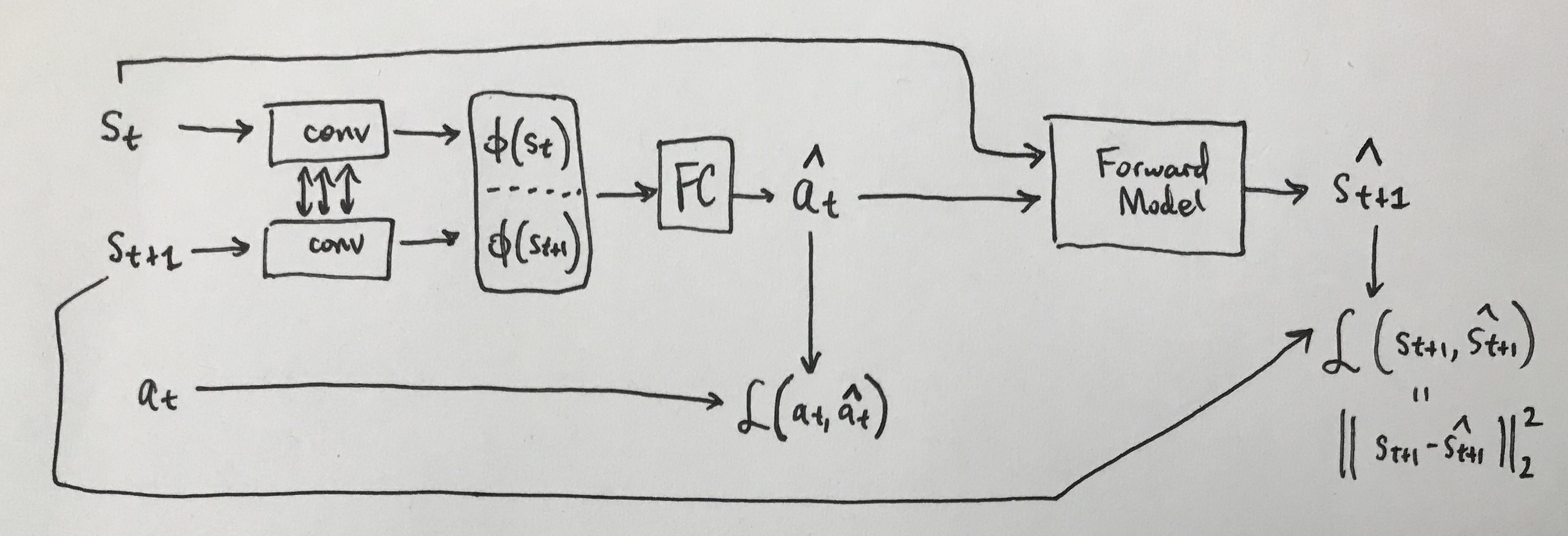
The basic one-step model, assuming that our inverse model just needs to predict
one action. The convolutional layers for the inverse model use the same tied
network convolutional weights. The action loss is the cross-entropy loss
(assuming discrete actions), and is not written in detail due to cumbersome
notation.
The main novelty here is that our predicted action \(\hat{a}_t\) from the inverse model is provided as input to the forward model, along with the current state \(s_t\). We then try and obtain \(s_{t+1}\), the actual state that was encountered during the agent’s exploration. This loss \(\mathcal{L}(s_{t+1}, \hat{s}_{t+1})\) is the standard Euclidean distance and is added with the action prediction loss \(\mathcal{L}(a_t,\hat{a}_t)\) which is the usual cross-entropy (for discrete actions).
Why is this extra loss function from the successor states used? It’s because we mostly don’t care which action we took, so long as it leads to the desired next state. Thus, we really want \(\hat{s}_{t+1} \approx s_{t+1}\).
Two extra long-ended comments:
-
There’s some subtlety with making this work. The state loss \(\mathcal{L}(s_{t+1}, \hat{s}_{t+1})\) treats \(s_{t+1}\) as ground truth, but that assumes we took action \(a_t\) from state \(s_t\). If we instead took \(\hat{a}_t\) from \(s_t\), and \(\hat{a}_t \ne a_t\), then it seems like the ground-truth should no longer be \(s_{t+1}\)?
Assuming we’ve trained long enough, then I understand why this will work, because the inverse model will predict \(\hat{a}_t = a_t\) most of the time, and hence the forward model loss makes sense. But one has to get to that point first. In short, the forward model training must assume that the given action will actually result in a transition from \(s_t\) to \(s_{t+1}\).
The authors appear to mitigate this with pre-training the inverse and forward models separately. Given ground truth data \(\mathcal{D} = \{s_1,a_1,s_2,\ldots,s_N\}\), we can pre-train the forward model with this collected data (no action predictions) so that it is effective at understanding the effect of actions.
This would also enable better training of the inverse model, which (as the authors point out) depends on an accurate forward model to be able to check that the predicted action \(\hat{a}_t\) has the desired effect in state-space. The inverse model itself can also be pre-trained entirely on the ground-truth data while ignoring \(\mathcal{L}(s_{t+1}, \hat{s}_{t+1})\) from the training objective.
I think this is what the authors did, though I wish there were a few more details.
-
A surprising aspect of the forward model is that it appears to predict the raw states \(s_{t+1}\), which could be very high-dimensional. I’m surprised that this works, given that (Agrawal et al., 2016) explicitly avoided this by predicting lower-dimensional features. Perhaps it works, but I wish the network architecture was clear. My guess is that the forward model processes \(s_t\) to be a lower dimensional vector \(\psi(s_t)\), concatenates it with \(\hat{a}_t\) from the inverse model, and then up-samples it to get the original image. Brandon Amos describes up-sampling in his excellent blog post. (Note: don’t call it “deconvolution.”)
Now how do we extend this for multi-step trajectories? The solution is simple: make the inverse model a recurrent neural network. That’s it. The model still predicts \(\hat{a}_t\) and we use the same loss function (summing across time steps) and the same forward model. For the RNN, the convolutional layers \(\phi\) take in the current state but they always take in \(s_g\), the goal state. They also take in \(h_{i-1}\) and \(a_{i-1}\) the previous hidden unit and the previous action (not the predicted action, that would be a bit silly when we have ground truth).
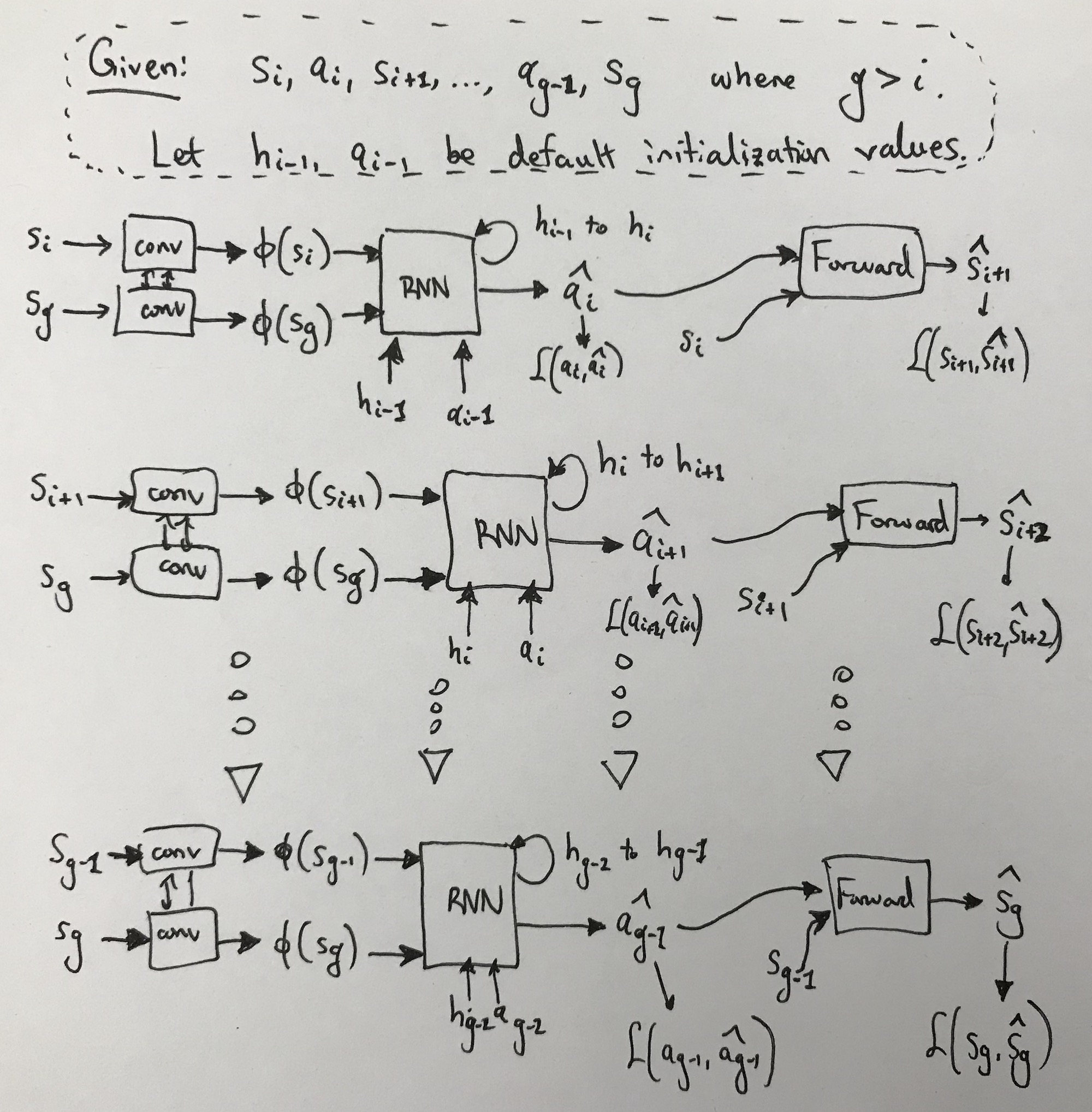
The multi-step trajectory case, visualizing several steps out of many.
Thoughts:
-
Why not make the forward model recurrent?
-
Should we weigh shorter-term actions highly instead of summing everything equally as they appear to be doing?
-
How do we actually decide the length of the action vector to predict? Or said in a better way, when do we decide that we’ve attained \(s_g\)?
Fortunately, the authors answer that last thought by training a deep neural network that can learn a stopping criterion. They say:
We sample states at random, and for every sampled state make positives of its temporal neighbors, and make negatives of the remaining states more distant than a certain margin. We optimize our goal classifier by cross-entropy loss.
So, states “close” to each other are positive samples, whereas “father” samples are negative. Sure, that makes sense. By distance I assume simple Euclidean distance on raw pixels? I’m generally skeptical of Euclidean distance but it might be necessary if the forward model also optimizes the same objective. I also assume this is applied after each time step, testing whether \(s_i\) at time \(i\) has reached \(s_g\). Thus, it is not known ahead of time how many actions the RNN must be able to predict before the goal is reset.
An alternative is mentioned about treating stopping as an action. There’s some resemblance to this and DDO’s option termination criterion.
Additionally, we have this relevant comment on OpenReview:
The independent goal recognition network does not require any extra work concerning data or supervision. The data used to train the goal recognition network is the same as the data used to train the PSF. The only prior we are assuming is that nearby states to the randomly selected states are positive and far away are negative which is not domain specific. This prior provides supervision for obtaining positive and negative data points for training the goal classifier. Note that, no human supervision or any particular form of data is required in this self-supervised process.
Yes, this makes sense.
Now let’s discuss the experiments. The authors test several ablations of their model:
-
An inverse model with no forward model at all (Nair et al., 2017). This is different from their earlier paper which used a forward model for regularization purposes (Agrawal et al., 2016). The model in (Nair et al., 2017) just used the inverse model for predicting an action given current image \(I_t\) and (critically!) a goal image \(I_{t+1}'\) specified by a human.
-
A more sophisticated inverse model with an RNN, but no forward model. Think of my most recent hand-drawn figure above, except without the forward portion. Furthermore, this baseline also does not use the action \(a_i\) as input to the RNN structure.
-
An even more sophisticated model where the action history is now input to the RNN. Otherwise, it is the same as the one I just described above.
Thus, all three of their ablations do not use the forward consistency model and are solely trained by minimizing \(\mathcal{L}(a_t,\hat{a}_t)\). I suppose this is reasonable, and to be fair, testing these out in physical trials takes a while. (Training should be less cumbersome because data collection is the bottleneck. Once they have data, they can train all of their ablations quickly.) Finally, note that all these inverse models take \((s_t,s_g)\) as input, and \(s_g\) is not necessarily \(s_{t+1}\). This, I remember from the greedy planner in (Agrawal et al., 2016).
The experiments are: navigating a short mobile robot throughout rooms and performing rope manipulation with the same setup from (Nair et al., 2017).
-
Indoor navigation. They show the model an image of the target goal, and check if the robot can use it to arrive there. This obviously works best when few actions are needed; otherwise, waypoints are necessary. However, for results to be interesting enough, the target image should not have any overlap with the starting image.
The actions are: (1) forward 10cm, (2) turn left, (3) turn right, and (4) standing still. They use several “tricks” such as using action repeats, applying a reset maneuver, etc. A ResNet acts as the image processing pipeline, and then (I assume) the ResNet output is fed into the RNN along with the hidden layer and action vector.
Indeed, it seems like their navigating robot can reach goal states and is better than the baselines! They claim their robot learns first to turn and then to move to the target. To make results more impressive, they tested all this on a different floor from where the training data was collected. Nice! The main downside is that they conducted only eight trials for each method, which might not be enough to be entirely convincing.
Another set of experiments tests imitation learning, where the goal images are far away from the robot, thus mandating a series of checkpoint images specified by a human. Every fifth image in a human demonstration was provided as a waypoint. (Note: this doesn’t mean the robot will take exactly five steps for each waypoint even if it was well trained, because it may take four or six or some other number of actions before it deems itself close enough to the target.) Unfortunately, I have a similar complaint as earlier: I wish there were more than just three trials.
-
Rope manipulation. They claim almost a 2x performance boost over (Nair et al., 2017) while using the same training data of 60K-70K interaction pairs. That’s the benefit of building upon prior work. They surprisingly never say how many trials they have, and their table reports only a “bootstrapped standard deviation”. Looking at (Nair et al., 2017), I cannot find where the 35.8% figure comes from (I see 38% in that paper but that’s not 35.8%…).
According to OpenReview comments they also trained the model from (Agrawal et al., 2016) and claim 44% accuracy. This needs to be in the final version of the paper. The difference from (Nair et al., 2017) is that (Agrawal et al., 2016) jointly train a forward model (but not to enforce dynamics but just as a regularizer), while (Nair et al., 2017) do not have any forward model.
Despite the lack of detail in some areas of the paper, (where’s the appendix?!?) I certainly enjoyed reading it and would like to try out some of this stuff.