Three Approaches to Deep Learning for Robotic Grasping
In ICRA 2018, “Deep Learning” was the most popular keyword in the accepted papers, and for good reason. The combination of deep learning and robotics has led to a wide variety of impressive results. In this blog post, I’ll go over three remarkable papers that pertain to deep learning for robotic grasping. While the core idea remains the same — just design a deep network, get appropriate data, and train — the papers have subtle differences in their proposed methods that are important to understand. For these papers, I will attempt to describe data collection, network design, training, and deployment.
Paper 1: Supersizing Self-supervision: Learning to Grasp from 50K Tries and 700 Robot Hours
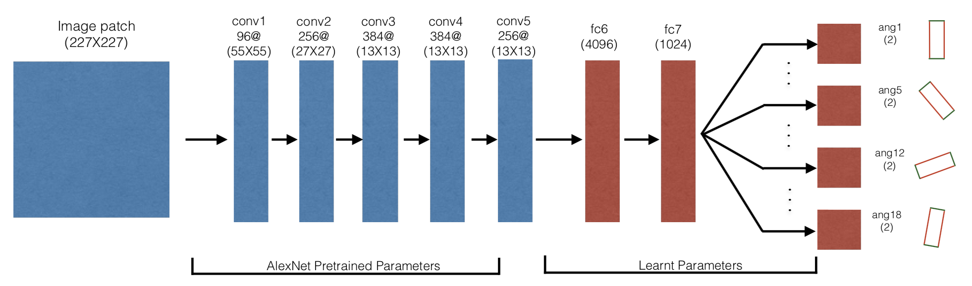 The grasping architecture used in this paper. No separate motor command is
passed as input to the network, since the position is known from the image patch
and the angle is one of 18 different discretized values.
The grasping architecture used in this paper. No separate motor command is
passed as input to the network, since the position is known from the image patch
and the angle is one of 18 different discretized values.
In this award-winning ICRA 2016 paper, the authors propose a data-driven grasping method that involves a robot (the Baxter in this case) repeatedly executing grasp attempts and training a network using automatically-labeled data of grasp success. The Baxter attempted 50K grasps which took 700 robot hours. Yikes!
-
Data Collection. Various objects get scattered across a flat workspace in front of the robot. An off-the-shelf “Mixture of Gaussians subtraction algorithm” is used to detect various objects. This is a necessary bias in the procedure so that a random (more like “semi-random”) grasp attempt will be near the region of the object and thus may occasionally succeed. Then, the robot moves its end-effector to a known height above the workspace, and attempts to grasp by randomly sampling a nearby 2D point and angle. To automatically deduce the success or failure label, the authors measure force readings on the gripper; if the robot has grasped successfully, then the gripper will not be completely closed. Fair enough!
-
Network Architecture. The neural network is designed to regress the grasping problem as an 18-way binary classification task (i.e., success or failure) over image patches. The 18-way branch at the end is because multiple angles may lead to successful grasps for an object, so it makes no sense to try and say only one out of 18 (or whatever the discretization) will work. Thus, they have 18 different logits, and during training on a given training data sample, only the branch corresponding to the angle in that data sample is updated with gradients.
They use a 380x380 RGB image patch centered at the target object, and downsample it to 227x227 before passing it to the network. The net uses fine-tuned AlexNet CNN layers pre-trained on ImageNet. They then add fully connected layers, and branch out as appropriate. See the top image for a visual.
In sum, the robot only needs to output a grasp that is 3 DoF: the \((x,y)\) position and the grasp angle \(\theta\). The \((x,y)\) position is implicit in the input image, since it is the central point of the image.
-
Training and Testing Procedure. Their training formally involves multiple stages, where they start with random trials, train the network, and then use the trained network to continue executing grasps. For faster training, they generate “hard-negative” samples, which are data points that the model thinks are graspable but are not. Effectively, they form a curriculum.
For evaluation, they can first measure classification performance of held-out data. This requires a forward pass for the grasping network, but does not require moving the robot, so this step can be done quickly. For deployment, they can sample a variety of patches, and for each, obtain the logits from the 18 different heads. Then for all those points, the robot picks the patch and angle combination that the grasp network rates as giving the highest probability of success.
Paper 2: Learning Hand-Eye Coordination for Robotic Grasping with Deep Learning and Large-Scale Data Collection
(Note that I briefly blogged about the paper earlier this year.)
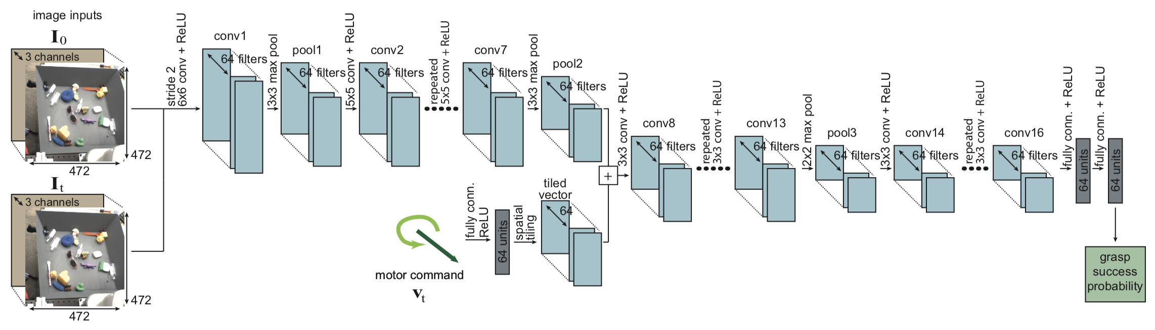 The grasping architecture used in this paper. Notice that it takes two RGB
images as input, representing the initial and current images for the grasp
attempt.
The grasping architecture used in this paper. Notice that it takes two RGB
images as input, representing the initial and current images for the grasp
attempt.
This paper is the “natural” next step, where we now get an order of magnitude more data points and use a much deeper neural network. Of course, there are some subtle differences with the method which are worth thinking about, and which I will go over shortly.
-
Data Collection. Levine’s paper uses six to fourteen robots collecting data in parallel, and is able to get roughly 800K grasp attempts over the course of two months. Yowza! As with Pinto’s paper, the human’s job is only to restock the objects in front of the robot (this time, in a bin with potential overlap and contact) while the robot then “randomly” attempts grasps.
The samples in their training data have labels that indicate whether a grasp attempt was successful or not. Following the trend of self-supervision papers, these labels are automatically supplied by checking if the gripper is closed or not, which is similar to what Pinto did. There is an additional image subtraction test which serves as a backup for smaller objects.
A subtle difference with Pinto’s work is that Pinto detected objects via a Mixture of Gaussians test and then had the robot attempt to grasp it. Here, the robot simply grasps at anything, and a success is indicated if the robot grasps any object. In fact, from the videos, I see that the robot can grasp multiple objects at once.
In addition, grasps are not executed in one shot, but via multiple steps of motor commands, ranging from \(T=2\) to \(T=10\) different steps. Each grasp attempt \(i\) provides \(T\) training data instances: \(\{(\mathbf{I}_t^i, \mathbf{p}_T^i - \mathbf{p}_t^i, \ell_i)\}_{t=1}^T\). So, the labels are the same for all data points, and all that matters is what happened after the last motor command. The paper discusses the interesting interpretation as reinforcement learning, which assumes actions induce a transitive relation between states. I agree in that this seems to be simpler than the alternative of prediction based on movement vectors at consecutive time steps.
-
Network Architecture. The paper uses a much deep convolutional neural network. Seriously, did they need all of those layers? I doubt that. But anyway, unlike the other architectures here, it takes two RGB 472x472x3 images as input (actually, both are 512x512x3 but then get randomly cropped for translation invariance), one for the initial scene before the grasp attempt, and the other for the current scene. The other architectures from Pinto and Mahler do not need this because they assume precise camera calibration, which allows for an open loop grasp attempt upon getting the correct target and angle.
In addition to the two input images, it takes in a 5D motor command, which is passed as input later on in the network and combined, as one would expect. This encodes the angle, which avoids the need to have different branches like in Pinto’s network. Then, the last part of the network predicts if the motor command will lead to (any) successful grasp (of any object in the bin).
-
Training and Testing Procedure. They train the network over the course of two months, updating the network 4 times and then increasing the number of steps for each grasp attempt from \(T=2\) to \(T=10\). So it is not just “collect and train” once. Each robot experienced different wear and tear, which I can agree with, though it’s a bit surprising that the paper emphasizes this a lot. I would have thought Google robots would be relative high quality and resistant to such forces.
For deploying the robot, they use a continuous servoing mechanism to continually adjust the trajectory solely based on visual input. So, the grasp attempt is not a single open-loop throw, but involves multiple steps. At each time step, it samples a set of potential motor commands, which are coupled with heuristics to ensure safety and compatibility requirements. The motor commands are also projected to go downwards to the scene, since this more closely matches the commands seen in the training data. Then, the algorithm queries the trained grasp network to see which one would have the highest success probability.
Levine’s paper briefly mentions the research contribution with respect to Dex-Net (coming up next):
Aside from the work of Pinto & Gupta (2015), prior large-scale grasp data collection efforts have focused on collecting datasets of object scans. For example, Dex-Net used a dataset of 10,000 3D models, combined with a learning framework to acquire force closure grasps.
With that, let’s move on to discussing Dex-Net.
Paper 3: Dex-Net 2.0: Deep Learning to Plan Robust Grasps with Synthetic Point Clouds and Analytic Grasp Metrics
(Don’t forget to check out Jeff Mahler’s excellent BAIR Blog post.)
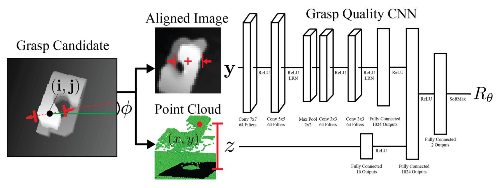 The grasping architecture used in this paper. Notice how the input image to the
far left is cropped and aligned to form the actual input to the GQ-CNN.
The grasping architecture used in this paper. Notice how the input image to the
far left is cropped and aligned to form the actual input to the GQ-CNN.
The Dexterity Network (“Dex-Net”) is an ongoing project at UC Berkeley’s AUTOLAB, led by Professor Ken Goldberg. There are a number of Dex-Net related papers, and for this post I will focus on the RSS 2017 paper since that uses a deep network for grasping. (It’s also the most cited of the Dex-Net related papers, with 80 as of today.)
-
Data Collection. Following their notation, states, grasps, depth images, and success metrics are denoted as \(\mathbf{x}\), \(\mathbf{u}\), \(\mathbf{y}\), and \(S(\mathbf{u},\mathbf{x})\), respectively. You can see the paper for the details. Grasps are parameterized as \(\mathbf{u} = (\mathbf{p}, \phi)\), where \(\mathbf{p}\) is the center of the grasp with respect to the camera pose and \(\phi\) is an angle in the table plane, which should be similar to the angle used in Pinto’s paper. In addition, depth images are also referred to as point clouds in this paper.
The Dex-Net 2.0 system involves the creation of a synthetic dataset of 6.7 million points for training a deep neural network. The dataset is created from 10K 3D object models from Dex-Net 1.0, and augmented with sampled grasps and robustness metrics, so it is not simply done via “try executing grasps semi-randomly.” More precisely, they sample from a graphical model to generate multiple grasps and success metrics for each object model, with constraints to ensure sufficient coverage over the model. Incidentally, the success metric is itself evaluated via another round of sampling. Finally, they create depth images using standard pinhole camera and projection models. They further process the depth images so that it is cropped to be centered at the grasp location, and rotated so that the grasp is at the middle row of the image.
Figure 3 in the paper has a nice, clear overview of the dataset generation pipeline. You can see the example images in the dataset, though these include the grasp overlay, which is not actually passed to the network. It is only for our human intuition.
-
Network Architecture. Unlike the two other papers I discuss here, the GQ-CNN takes in a depth image as input. The depth images are just 32x32 in size, so the images are definitely smaller as compared to the 227x227x3 in Pinto’s network, which in turn is smaller than the 472x472x3 input images for Levine’s network. See the image above for the GQ-CNN. Note the alignment of the input image; the Dex-Net paper claims that this removes the need to have a predefined set of discretized angles, as in Pinto’s work. It also arguably simplifies the architecture by not requiring 18 different branches at the end. The alignment process requires two coordinates of the grasp point \(\mathbf{p}\) along with the angle \(\phi\). This leaves \(z\), the height, which is passed as a separate layer. This is interesting, so instead of passing in a full grasp vector, three out of its four components are implicitly encoded in the image alignment process.
-
Training and Testing Procedure. The training seems to be straightforward SGD with momentum. I wonder if it is possible to use a form of curriculum learning as with Pinto’s paper?
They have a detailed experiment protocol for their ABB YuMi robot, which — like the Baxter — has two arms and high precision. I like this section of the paper: it’s detailed and provides a description for how objects are actually scattered across the workspace, and discusses not just novel objects but also adversarial ones. Excellent! In addition, they only define a successful grasp if the gripper held the object after not just lifting but also transporting and shaking. That will definitely test robustness.
The grasp planner assumes singulated objects (like with Pinto’s work, but not with Levine’s), but they were able to briefly test a more complicated “order fulfillment” experiment. In follow-up research, they got the bin-picking task to work.
Overall, I would argue that Dex-Net is unique compared to the two other papers in that it uses more physics and analytic-based prior methods to assist with Deep Learning, and does not involve repeatedly executing and trying out grasps.
In terms of the grasp planner, one could argue that it’s a semi-hybrid (if that makes sense) of the two other papers. In Pinto’s paper, the grasp planner isn’t really a planner: it only samples for picking the patches and then running the network to see the highest patch and angle combination. In Levine’s paper, the planner involves continuous visual servoing which can help correct actions. The Dex-Net setup requires sampling for the grasp (and not image patches) and, like Levine’s paper, uses the cross-entropy method. Dex-Net, though, does not use continuous servoing, so it requires precise camera calibration.
Update November 20, 2020: for a fourth way of doing this “deep learning and grasping” combination, check out my later post on how one can use fully convolutional neural networks for grasping. The advantage here is that execution time is faster, as it is not necessary to do any sampling of some sort, just a forward pass.