Machine learning for robotic manipulation is a popular research area, driven by the combination of larger datasets for robot grasping and the ability of deep neural networks to learn grasping policies from complex, image-based input, as I described in an earlier blog post. In this post, I review two papers from the same set of authors at MIT’s Robot Locomotion Group that deal with robotic manipulation. These papers use a concept that I was not originally familiar with: dense object descriptors. I’m glad I read these papers, because the application of dense object descriptors for robotic manipulation seems promising, and I suspect we will see a myriad of follow-up works in the coming years.

Paper 1: Dense Object Nets: Learning Dense Visual Object Descriptors By and For Robotic Manipulation (CoRL 2018)

This paper, by Florence, Manuelli, and Tedrake, introduced the use of dense descriptors in objects for robotic manipulation. It was honored with the best paper award at CoRL 2018 and got some popular, high-level press coverage.

The authors start the paper by wondering about the “right object representation for manipulation.” What does that mean? I view “representation” as the way that we encode data which we then pass as input to a machine learning (which means deep learning) algorithm. In addition, it would be ideal if this representation could be learned or formed in a “self supervised” manner. Self supervision is ideal for scaling up datasets, since it means manual labeling of the data is unnecessary. I’m a huge fan of self supervision, as evident by my earlier post on “self supervision” in machine learning and robotics.

The paper uses a dense object net to map a raw, full-resolution RGB image to a “descriptor image.” (Alternatively, we can call this network a dense descriptor mapping.) Concretely, say that function $f(\cdot)$ is the learned dense descriptor mapping. For an RGB image $I$, we have:

for some dimension $D$, which in this paper is usually $D=3$, but they test with some larger values, and occasionally with $D=2$.

I originally thought the definition of $f(I)$ must have had a typo. If we are trying to map a full resolution RGB image $I$ to some other “space” for machine learning, then surely we would want to decrease the size of the data, right? Ah, but after reading the paper carefully, I now understand that they need to keep the same height and width of the image to get pixel correspondences.

The function $f(I)$ maps each pixel in the original, three-channel image $I$, to a $D$-dimensional vector. The authors generally use $D=3$, and compared to larger values of $D$, using $D=3$ has the advantage in that descriptors can be visualized easily; it means the image is effectively another $H\times W\times 3$-dimensional image, so upon some normalization (such as to convert values into $[0,255]$) it can be visualized as a normal color image. This is explained in the accompanying video, and I will show a figure later from the paper.

What does the data and then the loss formulation look like for training $f$? The data consists of tuples with four elements: two images $I_a$ and $I_b$, then two pixels on the images, $u_a$ and $u_b$, respectively. Each pixel is therefore a 2-D vector in $\mathbb{R}^2$; in practice, each value in $u_a$ or $u_b$ can be rounded to the nearest pixel integer. We write $f(I_a)(u_a)$ for the channel values at pixel location $u_a$ in descriptor image $f(I_a)$. For example, if $f$ is the identity function and $I_a$ a pure white image, then $f(I_a)(u_a) = [255,255,255]$ for all possible values of $u_a$, because a white pixel value corresponds to 255 in all three channels.

There are two loss functions that add up to one loss function for the given image pair:

and

The final loss for $(I_a,I_b)$ is simply the sum of the two above:

Let’s deconstruct this loss function. Minimizing this loss will encourage $f$ to map pixels such that they are close in descriptor space with respect to Euclidean distance if they are matches, and far away — by at least some target margin $M$ — if they are non-matches. (We will discuss what we mean by matches and non-matches shortly.) The target margin was likely borrowed by the famous hinge loss (or “max margin” loss) that is used for training Support Vector Machine classifiers.

Here are two immediate, related thoughts:

• This is only for one image pair $(I_a,I_b)$. Surely we want more data, so while it isn’t explicitly stated in the paper, there must be an extra loop that samples for the image pair, and then samples the pixels in them.

• But how many pixels should we sample for a pair of images? The authors say they generate about one million pixel pairs! So, if we want to split our matches and non-matches roughly evenly, this just means $N_{\rm matches} \approx 500,000$ and $N_{\rm non-matches} \approx 500,000$. Thus, any two images provide a huge training data, since the data has to include pixels, and thus we can literally randomly draw the pixels from the two images.

To be clear on the credit assignment, the above math is not due to their paper, but actually from prior work (Schmidt et al., ICRA 2017). The authors of the CoRL 2018 paper use this formalism to apply it to robotic manipulation, and provide some protocols that accelerate training, to which we now turn.

The image above concisely represents several of the paper’s contributions with respect to improving the training process of descriptors, and particularly in the realm of robotic manipulation. Here, we are concerned with grasping various objects, so we want descriptors to be consistent among objects.

A match for images $I_a$ and $I_b$ at pixels $u_a$ and $u_b$ therefore means that the pixels located at $u_a$ and $u_b$ point to the same part of the object. A non-match is, well, basically everything else. In the image above, matching pairs of pixels are in green, and non-matching pairs are in red.

Mandatory “rant-like” side comment: I really wish the colors were different. Seriously, almost ANY other color pairing is better than red-green. I wish conference organizers could ban pairings of red-green in papers and presentations.

There are several problems with simply randomly drawing pixels $u_a$ and $u_b$. First, in all likelihood we will get a non-match (unless we have a really weird pair of images), and thus the training data is heavily skewed. Second, how do we ensure that matches are actually matches? We can’t have humans label manually, as that would be horrendously difficult and time-consuming.

Some of the related points and contributions they made were:

• By using prior work on 3D reconstruction and 3D change detection, the authors are able to isolate the pixels that correspond to the actual object. These pixels, whether or not they are matches (and it’s important to sample both matches and non-matches!), are usually more interesting than background pixels.

• It is beneficial to use domain randomization, but it should be done on the background so that the learned descriptors are not dependent on background to figure out locations and characteristics of objects. Note how the previous point about masking the object in the image enables background domain randomization.

• There are several strategies to enforce that the same function $f$ can apply to different object classes. An easy one is if images $I_a$ and $I_b$ have only one object each, and those objects are of different classes. Thus, every pair of sampled pixels among those two images is a non-match (as I believe all background pixels are considered non-matches).

There are a variety of additional contributions they make to the training process. I encourage you to read the paper to check out the details.

The majority of the experiments in the paper are for validating that the resulting descriptors make sense. By that, I mean that the descriptors are consistent across objects. For example, the same shoe, when seen from different camera perspectives, should have descriptors that are able to match the different components of the shoe.

The above image is illuminating. They use descriptors with $D=3$ and are able to visualize the descriptor images, shown in the second and fourth rows. Note that the colors in the descriptor images should not be interpreted in any way other than the fact that they indicate correspondence. That is, it would be equally appealing and satisfying to see the same descriptor images above, except with all the yellows replaced with greens, all the purples replaced with blue, and so on. What matters is that, among different images of the same object, we see the same color pattern for the objects (and ideally the background).

In addition, other ablation experiments show that their proposed improvements to the training process actually help. This is great stuff!

Their last experiment shows a real-world robot grasping objects. They are not learning a policy; given a target to grasp, they execute an open loop trajectory. What’s interesting from their experiment is that they can use descriptors to grasp the same part of an object (e.g., a shoe) even if the shoe is seen at different camera angles or from different positions. It even works when they use different shoes, since those still have the same general structure of a “shoe class” and thus descriptors can be consistent even among different class attributes.

Paper 2: Self-Supervised Correspondence in Visuomotor Policy Learning (arXiv 2019)

This paper can be viewed as a follow-up to the CoRL 2018 paper; unsurprisingly, it is by the same set of authors. Here, the focus is on using dense descriptors for training a visuomotor policy. (By “visuomotor” we mean a robot which sets “motor torques” based on image-based data.) The CoRL 2018 paper, in contrast, focused on simply getting accurate correspondences set up among objects in different images. You can find the arXiv version here and the accompanying project website here.

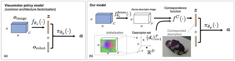
I immediately found something I liked in the paper. In the figure above, to the left, you see the most common way of designing a visuomotor policy. It involves passing the image through a CNN, and then getting a feature vector $\mathbf{z} \in \mathbb{R}^Z$. Then, it is concatenated with other non-image based information, such as end-effector information and relevant object poses. I believe this convention started with the paper by (Levine, Finn, et al., JMLR 2016), and indeed, it is very commonly used. For example, the Sim-to-Real cloth manipulation paper (Matas et al., CoRL 2018) used this convention. It’s nice when researchers think outside of the box to find a viable alternative.

Concretely, we get the action from the policy and the past set of observations via \(\mathbf{a}_t = \pi_\theta (\mathbf{o}_{0:t})\), and we have

representing the observation space. The usual factorization is:

where $Z$ is of much smaller dimensionality than the size of the full image $\mathbf{o}_{\rm image}$ (height times width times channels). This is a logical factorization that has become standard in the Deep Learning and Robotics literature.

Now, what is the main drawback of this approach? (There better be one, otherwise there would be no need to modify the architecture!) Florence and Manuelli argue that we should try and use correspondence information when training policies. Right now, doing end-to-end learning is popular, as are autoencoding methods, but why not explicitly enforce correspondence information? One can do this by enforcing $\mathbf{z}$ to encode pose information via setting an appropriate loss function with a target vector that has actual poses.

I was initially worried. Why not automatically learn $\mathbf{z}$ end-to-end? It seems risky to try and force $\mathbf{z}$ to have some representation. Poses, to be sure, are intuitively ideal, but if there’s anything machine learning has taught us over the past decade, it is probably that we should favor letting the data automatically determine latent features. The argument in the paper seems to be that learning intermediate representations (i.e., the descriptors) with surrogate objectives is better with less data, and that’s a fair point.

Prior work has not done this because:

• Prior work generally focuses on rigid objects, and pose estimation does not apply to deformable objects. I think “pose estimation” relies on assuming rigid objects. Knowing the 6 DoF pose of any point on the object means we know the full object configuration, assuming its shape is known beforehand.

• While other prior work interprets $\mathbf{z}$ as encoding spatial information, it is not trained directly for correspondence.

The authors propose directly using dense correspondence models in the learning process. They suggest four options, showing that a lot is up to discretion of the designer (but I don’t see any extensive comparisons among their four methods). Let there be a dense descriptor pre-trained model $f_{\theta_v}^{\rm dense}(\cdot)$ that was trained as in their CoRL 2018 paper. We have:

which provides the predicted location of descriptors and is used in three of their four proposed ways of incorporating correspondence with descriptors. We have $\mathbf{z} \in \mathbb{R}^{P \times D}$ where $P$ is the number of descriptors and $D$ is the descriptor dimension, usually two or three. Descriptors can be directly interpreted as 2D pixels or 3D coordinates, making $\mathbf{z}$ highly interpretable — a good thing as “interpretability” of feature vectors is something that everyone gets frustrated about in Deep Learning.

This raises an interesting question: how do we actually get \(\{d_1, \ldots, d_P\}\)? We can get a fixed reference image, say of the same object we’re considering, except in a different pose (that’s the whole point of using correspondences). Descriptors can also be optimized by backpropagation. Given the number of descriptors, which is a hyperparameter, the descriptors are combined with the image input to get $\mathbf{z}$. This “combination” is done with a “spatial softmax” operation. Like the normal softmax, the spatial softmax operation has no parameters but is differentiable. Hence, the objective used in the overall, outer loss function (which is behavior cloning, as the authors later describe) is used to pass though gradients via backpropagation, and then the spatial softmax is the local operation passing gradients back to the descriptors, which are directly adjusted via gradients. The spatial softmax operation is denoted with $f^C$, and the reference for it is attributed to (Levine, Finn, et al., JMLR 2016).

They combine correspondence with imitation learning, by using behavior cloning with a weighted average of $L_1$ and $L_2$ losses — pretty standard stuff. Remember again that for merging their work with descriptors, they don’t need to use behavior cloning, or imitation learning for that matter. It was probably just easiest for them to get interesting robotics results that way.

Their action space is

where \(\mathcal{A} = SE(3) \times \mathbb{R}^+\). For more details, see the paper.

Some of their other contributions have to do with the training process, such as proposing a novel data augmentation technique to prevent cascading errors, and a new technique for multi-camera time synchronized dense spatial correspondence learning. The latter is used to help train in dynamic environments, whereas the CoRL 2018 paper was limited to static environments.

They perform a set of simulated and then real experiments:

• Simulated Experiments: these involve using the DRAKE simulator. I haven’t used it before, but I want to learn about it. If it is not proprietary like MuJoCo, then perhaps the research community can migrate to it? They benchmark a variety of methods. (Strangely, some numbers are missing from Table I. I can understand why some are not tested, but not all of them.) They have many methods, with the differences arising from how each acquires $\mathbf{z}$. That’s the point of their experiments! Due to the simulated environments, they can encode ground truth positions and poses in $\mathbf{z}$ as an upper-bound baseline.

  The experiments show that their methods are better than prior work, and are nearly as good as the ones with ground truth in $\mathbf{z}$. There is also some nice analysis involving the convex hull of the training data (which is applicable because of the 2D nature of the table). If data is outside of that convex hull, then effectively we see an “out of distribution” data point, and hence policies have to generalize. Policies with 3D information seem to be better able to extrapolate outside the training distribution than those with only 2D information.

• Real-World Experiments: for these, they use a Kuka IIWA LBR robot with a parallel jaw gripper. As shown in the images below, they are able to get highly accurate descriptors. Essentially, one point on one object should be consistently labeled as the corresponding point on the object if it is in a different location, or if we use similar objects in the same class, such as using a different shoe type for descriptors trained on shoe-like objects.

They argue their method is better because they use correspondence — fair enough. For the experiment setup, their method is already near the limit of what can be achieved, since results are close to those of baselines with ground truth information in $\mathbf{z}$.

Closing Thoughts

Some thoughts and takeaways I have from reading these two papers above:

• Correspondence is a fundamental concept for computer vision. Because we want robots to learn things from raw images, it therefore seems logical that correspondence is also important for robotic manipulation. Correspondence will help us figure out how to manipulate objects in a similar way when they are oriented at different poses and perspectives.

• Self supervision is more scalable for large datasets than asking humans to manually label. Figuring out ways to automate labeling must be an important component of any proposed descriptor-based technique.

• I am still confused about how exactly we can get pixel correspondences via depth images, camera poses, and camera intrinsics, as described in the paper. It makes sense to me with some vague intuition, but I need to code and experience the full pipeline myself to actually understand.