More On Dense Object Nets and Descriptors: Applications to Rope Manipulation and Kit Assembly
In a prior blog post, I reviewed two papers about dense object descriptors in the context of robotic manipulation. The first paper, at CoRL (Florence et al., 2018), introduced it for object manipulation and open-loop grasping policies. The second paper, to appear at RA-Letters and ICRA (Florence et al., 2020), used descriptors and correspondence for policy optimization. In this post, I will discuss how descriptors can be used for two different robotics applications: rope manipulation and kit assembly. We can additionally combine descriptors with other tools in robotics such as imitation learning and self-supervision, which these papers demonstrate.
Before reading this post, I highly recommend going through the 30-minute PyTorch tutorial associated with the CoRL 2018 paper. I did not know anything about descriptors before reading the CoRL 2018 paper last year, and I appreciate the efforts of the authors to help us quickly learn the relevant concepts.
As a quick refresher on terminology, I refer to dense object nets as the networks which have descriptors as their output. They are “dense” because they involve predicting something at every pixel of an image. Don’t worry, this is not done by iterating through each target pixel (my brain hurts just thinking about doing that) but by passing the full image through the net and getting all the labels on each pixel in parallel.
Learning Rope Manipulation Policies Using Dense Object Descriptors Trained on Synthetic Depth Data
There is a whole sub-field of robotics that deals with rope manipulation. This paper, which recently came out of our lab at UC Berkeley, applies dense object descriptors for rope manipulation. They show, among other things, that descriptors can be applied to highly deformable objects. Previously, (Florence et al., 2018) applied it on slightly deformable objects, such as hats and shoes.
Another interesting aspect of this paper is that the authors train dense object nets in simulation. This provides perfect information of rope, so given two images of the same rope in different configurations, it should be possible to provide exact correspondences among pixels of the ropes. The paper argues that because rope is highly deformable, it is not sufficient to just change the pose of the camera to learn object descriptors, as was done in the earlier CoRL 2018 paper which used multiple camera views. I believe the CoRL paper needed to get multiple camera views for their full 3D reconstruction of the objects under consideration.
Blender is the simulator used in the paper. I know Blender reasonably well as we have recently used it for fabric manipulation (Seita et al., 2019). The below image shows a visualization of the simulator used in the work (left two columns).
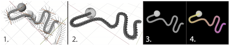
The third image shows a simulated depth image of the rope, where pixels are a height value from an overhead camera. The fourth image shows that we can define an ordering of points on the rope, where points close to the ball are closer to yellow, and the colors change as one “traverses” away from the rope. A couple of pointers:
- The simulator produces depth images, which may help in sim-to-real transfer since depth is naturally invariant to colors. We have been using depth for a lot of our papers, as we show in our 2018 BAIR Blog post. In addition to standard domain randomization techniques, the authors perform several tricks on the images of rope to make it look similar to the noisier depth images we encounter in practice.
- Regarding the color ordering on the rope, the goal in training a dense object net is to generate descriptors such that if we translate the descriptor values into pixels, we get a consistent color ordering among the same rope but in different configurations. All that matters is the relative ordering of colors. We don’t care if the descriptor network happens to “decide” that points closer to the ball are blue instead of yellow, so long as that “decision” is consistent among different images.
- There is a ball attached to one end of the rope, which is needed to enforce a notion of ordering among the pixels. Otherwise, there would be two possible orderings, which might fool a descriptor net. Indeed, the ablation studies show that this ball is perhaps the most important hyperparameter decision the authors made.
That was the simulator. We have to use it to get data to train the dense object network. The authors do this by sampling to get some rope state $\xi_1$. Then, they apply a random transformation to get $\xi_2$. This is essentially a robot’s action, defined as a pick and place transform. The pair is then used as a training data, where the goal is to train the dense object net to make corresponding points in $\xi_1$ and $\xi_2$ to be close to each other, while encouraging non-corresponding points to be further apart. The training loss is done in the same manner as in the CoRL 2018 paper so please read that paper for the exact loss function, which I also dissect in my prior post.
Here is a visualization of what descriptors learn:
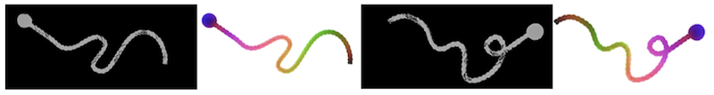
The first and third images show synthetic depth images of the rope in different configurations, and the second and fourth show visualizations of the corresponding dense object net outputs. Again, don’t get too caught up by the exact colors; all that matters is that they are consistent across the two images, and indeed they are! The process of generating these color images usually involves normalization techniques such as scaling the pixel values to be within $[0,255]$. In this paper, the descriptor dimension is 3, which makes it easy to visualize images.
You will also see that intersections and occlusions can be tricky with descriptors, since it may be impossible to get truly exact correlations; they would be restricted to pixels appearing at the uppermost layer of the object(s). The paper measures the uncertainty of descriptor nets and reports that, as expected, uncertainty is highest at intersections and occlusions.
The learned descriptors above are interesting, but now how do we use them in practice for robot manipulation? We need some benefit from descriptors, otherwise why we would use them? The paper reports two sets of experiments:
-
One-Shot Visual Imitation. No, don’t get confused with my post of a similar title, that was meta-learning, and here there is no meta-learning. The terminology means the robot is provided only one demonstration of a task to complete, where the demonstration is a sequence of images of rope states. The goal is to sequentially take actions to reach each of the images, or “sub-goals” if you prefer, in order. This is the same problem setting as in (Nair et al., 2017) – just think of it as requiring a demonstration at test time.
The policy is a greedy action: it uses descriptors from the current and (sub)goal images. From these, they sample paired points on the rope. They then look at the descriptor values, and find which pairing of sampled points is furthest from each other, and take a pick-and-place action to correct that. Intuitively, doing this each time gets the rope closer to the goal state because the greedy action has handled the most “distant” set of points. Assuming that actions do not cause any other descriptor pairs to increase in distance (a huge assumption!!) then eventually the rope has to look the same as in the human demonstration images.
-
Descriptor Parameterized Knot Tying. This is more specific for knot-tying, and uses a two-action sequence tuned towards a specific knot type. Thus, for another kind of knot they’d have to redefine the trajectory (and assume we already know how to do it) but there is no free lunch. They fix the actions for one rope, but here’s the clever part: they record the action vectors, but then “translate” that into descriptor space by passing it through the dense object net. This is what they mean by “defining an action in terms of descriptors.” Then, for a new goal image, since we already have the descriptors, we can use the original descriptor and map it into the corresponding pixels for the new goal image. We get the complete action by doing this for the pick and the place components. Thus, the action is generalizable across images.
For both experiments, they use a YuMi robot. For the former, they try and get the YuMi to manipulate the rope so it reaches some target, which they can measure with Intersection over Union (IoU). For the latter, they perform 50 knot-trying trials and report 66% success rates, out-performing prior work, but the caveat of course is that the experimental setup is not the same. I encourage you to visit the project website to see some videos.
There are also a set of simulated experiments that show extensive ablations over various perturbations of parameters. (If anything, I think there’s too many ablations and not enough focus on the robot experiments, but that’s probably a minor comment given the overall high quality of the paper.) The summary of the results is that descriptor quality, as measured on a held-out test set of images, is insensitive to a variety of parameters, with the exception of including a ball on one end or not. That is perfectly acceptable and reasonable.
To conclude, the advantages of the approach presented in the paper are that it uses depth and simulation to avoid the need for running real robots as in (Nair et al., 2017), and that the descriptors provide correspondence, allowing us to define interpretable, geometric actions. By that, I mean we can take a pixel location of a grasp point on a robot, and use descriptors to map that point to other rope configurations.
Form2Fit: Learning Shape Priors for Generalizable Assembly from Disassembly
This paper uses descriptors for a very different application: assembling kits together. The first author, Kevin Zakka, already has a nice blog post about the paper, so my post will try and dive more into the technical details.
Kit assembly is deliberately a broad topic, and applies to basically anything that involves packaging something. By using descriptors and machine learning, they can learn picking and placing actions which generalize to assembling other kits not seen in training. They argue that in assembly lines, kits may change every few weeks, motivating learning over hard-coded rules. I can see why Google might have wanted to do this because they might work with companies that have assembly lines.
My first reaction upon understanding the kit assembly task was: great, this is cool, and a problem that I wish I had thought about earlier, but how does one get data on assembling kits? That seems much harder to do in simulation or the real world compared to rope manipulation.
The authors cleverly get data by dis-assembly from complete kits, and then repeating the process in reverse to assemble complete kits, in a manner similar to time-reversal as self-supervision. Even if actions are not truly reversible, such as with a placing operation that displaces existing objects, it seems logical that this helps get more high-quality data since it is intuitively harder to assemble than to dis-assemble. Since the paper does not use simulators, the downside is that a human would have to first provide an assembled kit and then maybe manually assemble things should something go wrong in data collection. As long as this does not need to happen too frequently, then it is acceptable. They report that they need just 500 disassembly sequences, though this is per training kit (to be fair, there are not many training kits). That’s roughly on the order of how many data points I had to physically collect for our bed-making paper from ISRR 2019.
Here is an overview of the pipeline, caption included from the paper:
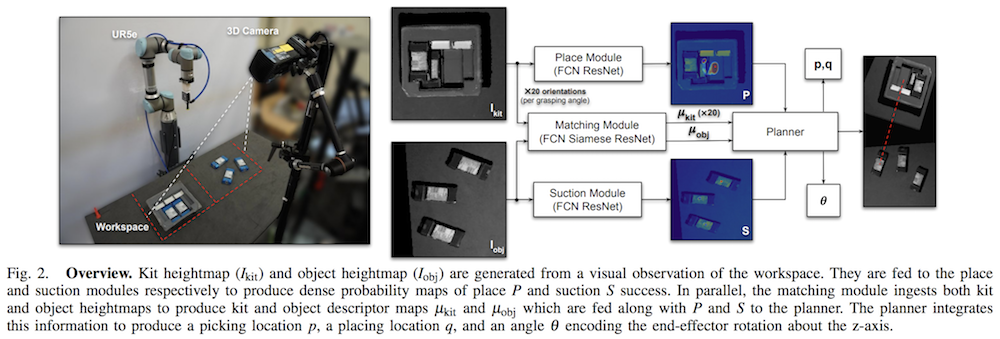
They use three fully convolutional neural networks in the pipeline. Recall that fully convolutional networks, which were introduced through a monumentally impactful paper from Trevor Darrell’s group a few years ago at Berkeley, are those that use only convolutional layers and efficiently perform dense per-pixel operations by mapping an image of size $(H\times W\times c_1)$ to another one of size $(H\times W\times c_2)$. Thus, all three networks produce per-pixel predictions of something with respect to the input image.
For kit assembly, the action space consists of a pick $p$, a place $q$, and an orientation for placement $\theta$. In addition, $p$ and $q$ are image pixels, which are then converted to a coordinate with respect to the robot’s base frame. The UR5 robot they use applies suctions, which reminds me of Jeff Mahler’s suctioning paper from ICRA 2018.
Interestingly, all three networks use depth images, like the rope manipulation paper above. However, the authors also use grayscale images and concatenate it with the depth images, producing “Grayscale-Depth” images (and not “RGB-Depth” images). I wonder why we don’t see more grayscale since that may reduce the need for heavy color-based domain randomization or additional training data?
The authors split the workspace into two images, one for showing the kit $I_{\rm kit}$ and the other for showing the objects $I_{\rm obj}$ which are initially scattered around and must be assembled in the kit.
Now let’s review the details of the three networks, which are called the suction, placing, and matching modules.
Suction module. For each pixel in $I_{\rm obj}$, this determines the success probability of grasping (i.e., suctioning) something.
- Getting labels is straightforward. The robot can measure the “airflow” of its suction gripper. For a given grasp point pixel $p$, if the airflow shows a success, then from the input image, we must encourage the suction network to assign pixel $p$ as a success. This is only one pixel out of many, so in practice the authors end up artificially increasing a radius about $p$ and labeling those a success. Notice that (a) sometimes we may get failures, so we’d do the same as earlier except assign a failure, and (b) other pixels backpropagate with zero loss. They do NOT assign other pixels as failures, because we don’t know if suctioning at other pixels far from $p$ could indeed lead to picking up something.
- The loss function uses the binary cross entropy loss, i.e., success or failure, for the pixels that were grasped, including those nearby as I mentioned earlier. Interestingly, the authors combine this with a “dice” loss. You can read the technical details in the paper but to summarize I believe it’s used to address class imbalance. For Form2Fit, I think because of the author’s setup, most of the suctions will be a success, and hence training is dominated by “pixel $p$ in a given image is a good pick point” rather than “pixel $p$ in a given image is a bad pick point.”
-
Finally, how does the data collection work from the time reversal? It’s pretty clever. First, when we disassemble, at each time we are given an image $I_{\rm kit}^{(t)}$ and apply suctioning on point $p^{(t)}$, where here I add the $t$ superscript to represent time. Notice that this is not the same as what happens during test time, where we must apply suctioning on images of objects, i.e., $I_{\rm obj}$ — but we can think of this as a clever form of data augmentation. Thus, the dis-assembly gives us a sequence of data which includes both picking from observations of the kit and placing where the objects will be during test time:
\[\{ (I_{\rm kit}^{(1)}, p^{(1)}), (I_{\rm obs}^{(1)}, q^{(1)}), (I_{\rm kit}^{(2)}, p^{(2)}), (I_{\rm obs}^{(2)}, q^{(2)}), \ldots \}\]Then, during the assembly process, we apply actions in reverse, this time looking at images $I_{\rm obj}^{(t)}$ at each time step, but with the placing action from earlier as the new suctioning action!
Place module. This network figures out a placing pixel into $I_{\rm kit}$, under the assumption that we are suctioning something from the suction network. A key design decision is that they discretize the angle into 20 groups, so there are 20 images passed through the placing network in parallel. Again, this is per-pixel, so for every pixel, there is a value that tells us the probability of placing success. Their deoderant kit example also shows how the placing module implicitly encodes ordering conditioned on the input image. The training process is similar to the suctioning network, with the exception that there isn’t a notion of getting a success signal via measuring something like suction airflow.
- The loss function also uses the cross entropy and a dice loss.
- For every pixel in $I_{\rm kit}$, we need to train the net so that it shows high success for successful places, and low success for failures. To get data, we once again use the time reversal sequence from above. Precisely, the labels are the suction location $p$ at time $t$ and the heightmap $I_{\rm kit}$ at $t+1$. Intuitively this is because if we do the sequence in reverse, we will have $I_{\rm kit}$ as the target with location $p$ as our placing point, i.e., $q$. These are the “success labels” since we assume that the suction step from the disassembly was a success, which seems reasonable since the authors can command the robot to grasp at “reasonable” coordinates on the kit.
Match module. This is the most interesting one to me because it uses descriptors. But first, why do we need this if we already have picking and placing? They argue:
While the suction and placing modules provide a list of candidate picking and placing locations, the system requires a third module to 1) associate each suction location on the object to a corresponding placing location in the kit and 2) infer the change in object orientation. This matching module serves as the core of our algorithm, which learns dense pixel-wise orientation-sensitive correspondences between the objects on the table and their placement locations in the kit.
This makes sense. What would happen if we did not have this network, and only relied on the placing network? It still has a set of 20 rotations as input, so I wonder what happens if we just take the highest probability among all pixels in all 20 images to satisfy (2)? I definitely agree, though, that we need a way to do (1) to get correspondence, because different objects should be placed at different locations.
We have $f: I \in \mathbb{R}^{H\times W\times 2} \to \mathbb{R}^{H\times W \times d}$. In this paper, the descriptor dimension is $d=64$. That is super large compared to the other paper on rope manipulation, and compared to the work from Russ Tedrake’s group. I’m surprised it is that high but I am sure the authors did extensive testing on the descriptor dimension, which they report in the supplementary material. It is a Siamese network with two fully convolutional residual streams, each sharing the same weights (since that’s what “Siamese network” means). The kit image $I_{\rm kit}$ maps to 20 separate descriptors, each of which are 64-dimensional, and one of them is selected to inform the change in rotation via:
\[\theta = \frac{360}{20} \times \arg\min_j \| \mu_{\rm kit}^{ij} - \mu_{\rm obj}^i\|_2^2 \quad {\rm for} \;\; j \in \{1,2,\ldots, 20\},\; i \in \{1,2,\ldots, H\times W\}\]The superscript of $j$ means we take one of the 20 descriptor images, so both descriptor images above, $\mu_{\rm kit}^j$ and $\mu_{\rm obj}$, are of dimension $(H\times W\times d)$. Then, we add the superscript of $i$ to represent a single pixel within those images, one of $H\times W$ candidate pixels. This way, we consider the best pixel match among all possible kit-object descriptor images. Finally, the $360/20$ fraction scales the index $j$ appropriately.
Now, how can we train the matching network to encourage similarity in both correspondence between picking and placing, and also the rotation? The loss function itself is the same as the one used in the CoRL 2018 paper, meaning that we need to sample matches and non-matches at the pixel level. The matches are taken from image pairs $(I_{\rm kit}, I_{\rm obj})$ where the kit image must be of the correct rotation (out of 20). Non-matches can be sampled from any of the 20 kit images. Within any pair of images, the pixel correspondences are labeled via object masks, which assumes that the rotation angle $\theta$ can provide us with the label of every pixel in the kit cavity and the corresponding pixel on the object, which is pulled outside the kit through data collection. This should work, particularly because the authors fix the kit to the surface; if that weren’t the case it might be harder to label correspondences.
Once the three networks are trained, the policy comes from the planner. It samples potential actions and then uses descriptors to see which pick-and-place pair (in descriptor space) have the lowest L2 distance, and that’s the action. Like with the rope manipulation paper, the policy is generally simple to describe and involves minimizing some distance in descriptors.
They conduct experiments using a physical UR5 robot, and evaluate by calculating the percentage of times when objects are placed into their target locations. I wonder if this involves some subjective interpretations, because I can imagine (and I see from the videos) that some objects might be almost but not quite inserted. As long as they are consistent with their interpretation, it is probably fine. The experiments show a number of promising results and effectiveness in assembling kits, with generalization to initial conditions of kits, and even to new kits entirely. They wrap up the results with a t-SNE visualization. Overall, I was really impressed with these results. Once again I encourage you to go to the project website for videos for a better understanding.
Conclusion
Hopefully this gives a readable overview of two different applications of dense object descriptors, showcasing the versatility of the technique. To be concrete, here are the papers I covered in this and my prior post, along with the original ICRA 2017 paper:
-
Tanner Schmidt, Richard Newcombe, Dieter Fox. Self-Supervised Visual Descriptor Learning for Dense Correspondence. ICRA 2017.
-
Peter Florence, Lucas Manuelli, Russ Tedrake. Dense Object Nets: Learning Dense Visual Object Descriptors By and For Robotic Manipulation. CoRL 2018.
-
Peter Florence, Lucas Manuelli, Russ Tedrake. Self-Supervised Correspondence in Visuomotor Policy Learning. RA-Letters and ICRA 2020.
-
Priya Sundaresan, Jennifer Grannen, Brijen Thananjeyan, Ashwin Balakrishna, Michael Laskey, Kevin Stone, Joseph E. Gonzalez, Ken Goldberg. Learning Rope Manipulation Policies Using Dense Object Descriptors Trained on Synthetic Depth Data. ICRA 2020.
-
Kevin Zakka, Andy Zeng, Johnny Lee, Shuran Song. Form2Fit: Learning Shape Priors for Generalizable Assembly. ICRA 2020.
Just like combining imitation learning and reinforcement learning or using simulators effectively with self-supervision, I think descriptors for correspondence belong in the toolkit we should use to develop general-purpose robots.