For at least a year, I’ve been a huge fan of the Deep Q-Network algorithm. It’s from Google DeepMind, and they used it to train AI agents to play classic Atari 2600 games at the level of a human while only looking at the game pixels and the reward. In other words, the AI was learning just as we would do!

Last year, I started a personal project related to DQNs and Atari 2600 games, which got me delving into the details of DeepMind’s two papers (from NIPS workshop 2013 and NATURE 2015). One thing that kept confusing me was how to interpret their frame skipping and frame processing steps, because each time I read their explanation in their papers, I realized that their descriptions were rather ambiguous. Therefore, in this post, I hope to clear up that confusion once and for all.

I will use Breakout as the example Atari 2600 game, and the reference for the frame processing will be from the NATURE paper. Note that the NATURE paper is actually rather “old” by deep learning research standards (and the NIPS paper is ancient!!), since it’s missing a lot of improvements such as Prioritized Experience Replay and Double Q-Learning, but in my opinion, it’s still a great reference for learning DQN, particularly because there’s a great open-source library which implements this algorithm (more on that later).

To play the Atari 2600 games, we generally make use of the Arcade Learning Environment library which simulates the games and provides interfaces for selecting actions to execute. Fortunately, the library allows us to extract the game screen at each time step. I modified some existing code from the Python ALE interface so that I could play the Atari games myself by using the arrow keys and spacebar on my laptop. I took 30 consecutive screenshots from the middle of one of my Breakout games and stitched them together to form the image below. It’s a bit large; right click on it and select “Open Image in New Tab” to see it bigger. The screenshots should be read left-to-right, up-to-down, just like if you were reading a book.

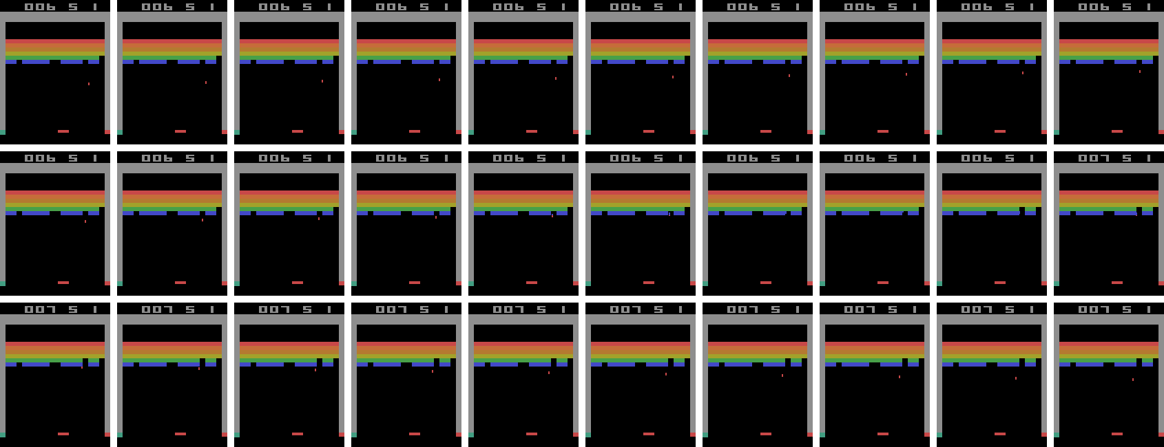
Note that there’s no reason why it had to be me playing. I could have easily extracted 30 consecutive frames from the AI playing the game. The point is that I just want to show what a sequence of frames would look like.

I saved the screenshots each time I executed an action using the ALE Python interface. Specifically, I started with ale = ALEInterface() and then after each call to ale.act(action), I used rgb_image = ale.getScreenRGB(). Thus, the above image of 30 frames corresponds to all of the screenshots that I “saw” while playing in the span of a half-second (though obviously no human would be able to distinguish among all 30 frames at once). In other words, if you save each screenshot after every action gets executed from the ALE python library, there’s no frame skipping.

Pro tip: if you haven’t modified the default game speed, play the game yourself, save the current game screenshot after every action, and check if the total number of frames is roughly equivalent to the number of seconds multiplied by 60.

Now that we have 30 consecutive in-game images, we need to process them so that they are not too complicated or high dimensional for DQN. There are two basic steps to this process: shrinking the image, and converting it into grayscale. Both of these are not as straightforward as they might seem! For one, how do we shrink the image? What size is a good tradeoff for computation time versus richness? And in the particular case of Atari 2600 games, such as in Breakout, do we want to crop off the score at the top, or leave it in? Converting from RGB to grayscale is also – as far as I can tell – an undefined problem, and there are different formulas to do the conversion.

For this, I’m fortunate that there’s a fantastic DQN library open-source on GitHub called deep_q_rl, written by Professor Nathan Sprague. Seriously, it’s awesome! Professor Sprague must have literally gone through almost every detail of the Google DeepMind source code (also open-source, but harder to read) to replicate their results. In addition, the code is extremely flexible; it has separate NIPS and NATURE scripts with the appropriate hyperparameter settings, and it’s extremely easy to tweak the settings.

I browsed the deep_q_rl source code to learn about how Professor Sprague did the downsampling. It turns out that the NATURE paper did a linear scale, thus keeping the scores inside the screenshots. That strikes me as a bit odd; I would have thought that cropping the score entirely would be better, and indeed, that seems to have been what the NIPS 2013 paper did. But whatever. Using the notation of (height,width), the final dimensions of the downsampled images were (84,84), compared to (210,160) for the originals.

To convert RGB images to grayscale, the deep_q_rl code uses the built-in ALE grayscale conversion method, which I’m guessing DeepMind also used.

The result of applying these two pre-processing steps to the 30 images above results in the new set of 30 images:

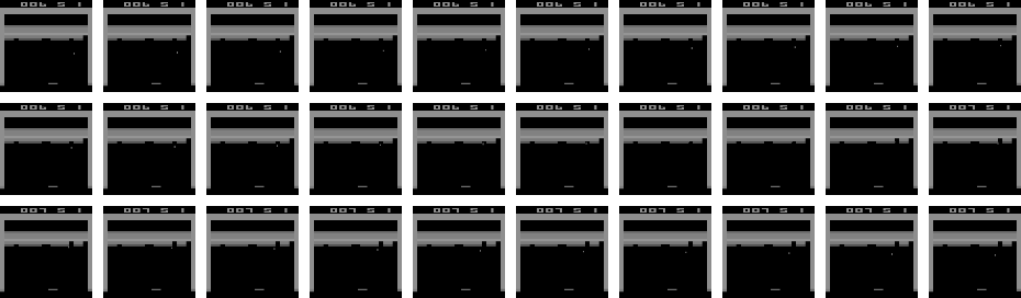
Applying this to all screenshots encountered in gameplay during DQN training means that the data dimensionality is substantially reduced, and also means the algorithm doesn’t have to run as long. (Believe me, running DQN takes a long time!)

We have all these frames, but what gets fed as input to the “Q-Network”? The NATURE and NIPS paper used a sequence of four game frames stacked together, making the data dimension (4,84,84). (This parameter is called the “phi length”) The idea is that the action agents choose depends on the prior sequence of game frames. Imagine playing Breakout, for instance. Is the ball moving up or down? If the ball is moving down, you better get the paddle in position to bounce it back up. If the ball is moving up, you can wait a little longer or try to move in the opposite direction as needed if you think the ball will eventually reach there.

This raises some ambiguity, though. Is it that we take every four consecutive frames? NOPE. It turns out that there’s a frame skipping parameter, which confusingly enough, the DeepMind folks also set at 4. What this means in practice is that only every fourth screenshot is considered, and then we form the “phi”s, which are the “consecutive” frames that together become the input to the neural network function approximator. Consider the updated sequence of screenshots, with the skipped frames denoted with an “X” over them:

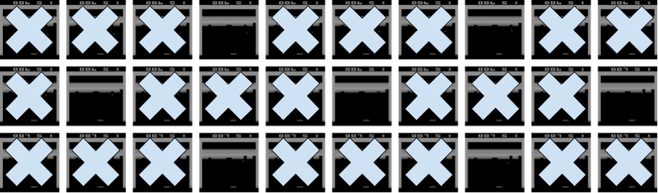
What ends up happening is that the states are four consecutive frames, ignoring all of the “X”-ed out screenshots. In the above image, there are only seven non-skipped frames. Let’s denote these as \(x_1,x_2,\ldots, x_7\). The DQN algorithm will use \(s_1 = (x_1,x_2,x_3,x_4)\) as one state. Then for the next state, it uses \(s_2 = (x_2,x_3,x_4,x_5)\). And so on.

Crucially, the states are overlapping. This was another thing that wasn’t apparent to me until I browsed Professor Sprague’s code. Did I mention I’m a huge fan of his code?

A remark before we move on: one might be worried that the agent is throwing away a lot of information using the above procedure. In fact, it actually makes a lot of sense to do this. Seeing four consecutive frames without subsampling doesn’t give enough information to discern motion that well, especially after the downsampling process.

There’s one more obscure step that Google DeepMind did: they took the component-wise maximum over two consecutive frames, which helps DQN deal with the problem of how certain Atari games only render their sprites every other game frame. Is this maximum done over all the game screenshots, or only the subsampled ones (every fourth)? It’s the former.

Ultimately, we end up with the revised image below:

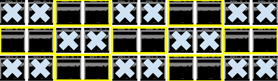
I’ve wrapped two consecutive screenshots in yellow boxes, to indicate that we’re taking the pixel-by-pixel (i.e. component-wise) maximum of the two images, which then get fed into as components for our states \(s_i\). Think of each of the seven yellow boxes above as forming one of the \(x_i\) frames. Then everything proceeds as usual.

Whew! That’s all I have to say regarding the pre-processing. If you want to be consistent with the NATURE paper, try to perform the above steps. There’s still a lot of ambiguity, unfortunately, but hopefully this blog post clarifies the major steps.

Aside from what I’ve discussed here, I want to bring up a few additional points of interest:

• OpenAI also uses the Atari 2600 games as their benchmark. However, when we perform an action using OpenAI, the action we choose is performed either 2, 3, or 4 frames in a row, chosen at random. These are at the granularity of a single, true game frame. To clarify, using our method above from the NATURE paper would mean that each action that gets chosen is repeated four times (due to four skipped game frames). OpenAI instead uses 2, 3, or 4 game frames to introduce stochasticity, but doesn’t use the maximum operator across two consecutive images. This means if I were to make a fifth image representing the frames that we keep or skip with OpenAI, it would look like the third image in this blog post, except the consecutive X’s would number 1, 2, or 3 in length, and not just 3. You can find more details in this GitHub issue.
• On a related note regarding stochasticity, ALE has an action repeat probability which is hidden to the programmer’s interface. Each time you call an action, the ALE engine will ignore (!!) the action with probability 25% and simply repeat the previous action. Again, you can find more discussion on the related GitHub issue.
• Finally, as another way to reduce stochasticity, it has become standard to use a human starts metric. This method, introduced in the 2015 paper Massively Parallel Methods for Deep Reinforcement Learning, suggests that humans play out the initial trajectory of the game, and then the AI takes over from there. The NATURE paper did something similar to this metric, except that they chose a random number of no-op actions for the computer to execute at the start of each game. That corresponds to their “no-op max” hyperparameter, which is described deep in the paper’s appendix.

Why do I spend so much time obsessing over these details? It’s about understanding the problem better. Specifically, what engineering has to be done to make reinforcement learning work? In many cases, the theory of an algorithm breaks down in practice, and substantial tricks are required to get a favorable result. Many now-popular algorithms for reinforcement learning are based on similar algorithms invented decades ago, but it’s only now that we’ve developed the not just the computational power to run them at scale, but also the engineering tricks needed to get them working.

As I mentioned in my review on Berkeley’s Deep Reinforcement Learning class, I have been wanting to write more about reinforcement learning, so in this post, I will provide some comments on Q-Learning and Linear Function Approximation. I’m hoping these posts can serve as another set of brief RL introductions, similar to Andrej’s excellent post on deep RL.

Last year, I wrote an earlier post on the basics of MDPs and RL. This current one serves as the continuation of that by discussing how to scale RL into settings that are more complicated than simple tabular scenarios but nowhere near as challenging as, say, learning how to play Atari games from high-dimensional input. I won’t spend too much time trying to labor though the topics in this post, though. I want to save my effort for the deep variety, which is all the rage nowadays and a topic which I hope to eventually write a lot about for this blog.

To hep write this post, here are two references I used to quickly review Q-Learning with function approximation.

1. Tutorial on RL and Linear Function Approximators
2. Barto and Sutton’s RL book, in HTML

I read (1) entirely, and (2) only partly, since it is, after all, a full book (note that the authors are in the process of making a newer edition!). Now let’s move on to discuss an important concept: value iteration with function approximation.

Value Iteration with Function Approximation

Value Iteration is probably the first RL-associated algorithm that students learn. It lets us assign values \(V(s)\) to states \(s\), which can then be used to determine optimal policies. I explained the algorithm in my earlier post, but just to be explicit, here’s a slide from my CS 287 class last fall which describes the procedure:

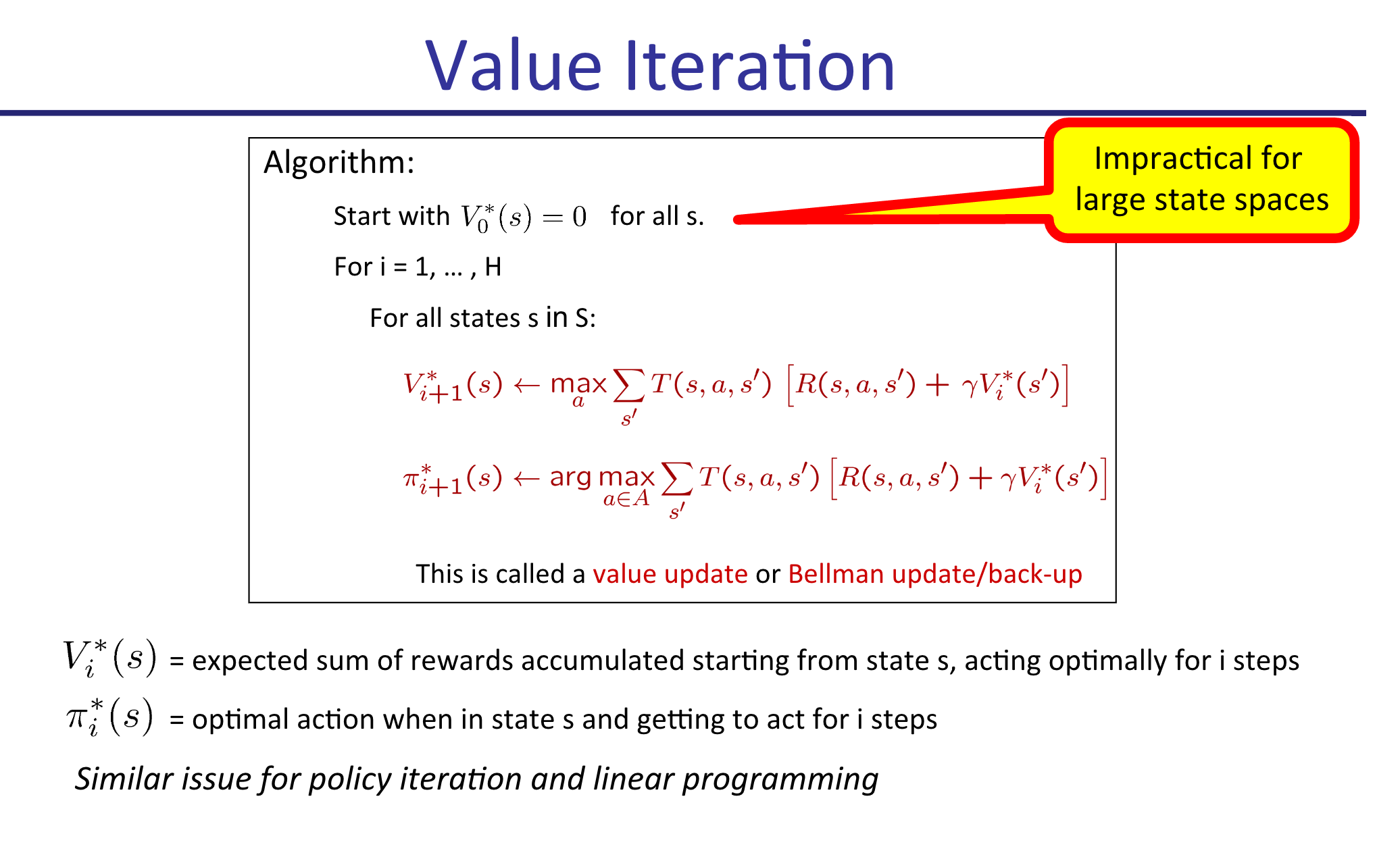
Looks pretty simple, right? For each iteration, we perform updates on our values \(V_{i}^*\) until convergence. Each iteration, we can also update the policy \(\pi_i^*\) for each state, if desired, but this is not the crucial part of the algorithm. In fact, since the policy updates don’t impact the \(V_{i+1}^*(s)\) max-operations in the algorithm (as shown above), we can forget about updating \(\pi\) and do that just once after the algorithm has converged. This is what Barto and Sutton do in their Value Iteration description.

Unfortunately, as suggested by the slide, (tabular) Value Iteration this is not something we can do in practice beyond the simplest of scenarios due to the curse of dimensionality in \(s\). Note that \(a\) is not usually a problem. Think of \(9 \times 9\) Go, for instance: according to reference (1) above, there are \(|\mathcal{S}| = 10^{38}\) states, but just \(|\mathcal{A}| = 81\) actions to play. In Atari games, the disparity is even greater, with far more states but perhaps just two to five actions per game.

The solution is to obtain features and then represent states with a simple function of those features. We might use a linear function, meaning that

where \(\theta_0\) is a bias term with 1 “absorbed” into \(\phi\) for simplicity. This function approximation dramatically reduces the size of our state space from \(|\mathcal{S}|\) into “\(|\Theta|\)” where \(\Theta\) is the domain for \(\theta \in \mathbb{R}^n\). Rather than determining \(V_{i+1}^*(s)\) for all \(s\), each iteration our goal is to instead update the weights \(\theta_i\).

How do we do that? The most straightforward way is to reformulate it as a supervised learning problem. From the tabular version above, we know that the weights should satisfy the Bellman optimality conditions. We can’t use all the states for this update, but perhaps we can use a small subset of them?

This motivates the following algorithm: each iteration \(i\) in our algorithm with current weight vector \(\theta^{(i)}\), we sample a very small subset of the states \(S' \subset S\) and compute the official one-step Bellman backup updates:

Then we find the next set of weights:

which can be done using standard supervised learning techniques. This is, in fact, an example of stochastic gradient descent.

Before moving on, it’s worth mentioning the obvious: the performance of Value Iteration with function approximation is going to depend almost entirely on the quality of the features (along with the function representation, i.e. linear, neural network, etc.). If you’re programming an AI to play PacMan, the states \(s\) will be the game board, which is far too high-dimensional for tabular representations. Features will ideally represent something relevant to PacMan’s performance in the game, such as the distance to the nearest ghost, the distance to the nearest pellet, whether PacMan is trapped, and so on. Don’t neglect the art and engineering of feature selection!

Q-Learning with Function Approximation

Value Iteration with function approximation is nice, but as I mentioned in my last post, what we really want in practice are \(Q(s,a)\) values, due to the key fact that

which avoids a costly sum over the states. This will cost us extra in the sense that we have to now use a function with respect to \(a\) in addition to \(s\), but again, this is not usually a problem since the set of actions is typically much smaller than the set of states.

To use Q-values with function approximation, we need to find features that are functions of states and actions. This means in the linear function regime, we have

What’s tricky about this, however, is that it’s usually a lot easier to reason about features that are only functions of the states. Think of the PacMan example from earlier: it’s relatively easy to think about features by just looking at what’s on the game grid, but it’s harder to wonder about what happens to the value of a state assuming that action \(a\) is taking place.

For this reason, I tend to use the following “dimension scaling trick” as recommended by reference (1) above, which makes the distinction between different actions explicit. To make this clear, image an MDP with two features and four actions. The features for state-action pair \((s,a_i)\) can be encoded as:

Why the need to use different feature for different actions? Intuitively, if we didn’t do this (and kept \(\phi(s,a)\) with just two non-bias features) then the action would have no effect! But actions do have impacts on the game. To use the PacMan example again, imagine that the PacMan agent has a pellet to its left, so the agent is one move away from being invincible. At the same time, however, there could be a ghost to PacMan’s right! The action that PacMan takes in that state (LEFT or RIGHT) will have a dramatic impact on the resulting reward obtained! It is therefore important to take the actions into account when featurizing Q-values.

As a reminder before moving on, don’t forget the bias term! They are necessary to properly scale the function values independently of the features.

Online Least Squares Justification for Q-Learning

I now want to sketch the derivation for Q-Learning updates to provide intuition for why it works. Knowing this is also important to understand how the training process works for the more advanced Deep-Q-Network algorithm/architecture.

Recall the standard Q-Learning update without function approximation:

Why does this work? Imagine that you have some weight vector \(\theta^{(i)}\) at iteration \(i\) of the algorithm and you want to figure out how to update it. The standard way to do so is with stochastic gradient descent, as mentioned earlier in the Value Iteration case. But what is the loss function here? We need that so we can compute the gradient.

In Q-Learning, when we approximate a state-action value \(Q(s,a)\), we want it to be equal to the reward obtained, plus the (appropriately discounted) value of playing optimally from thereafter. Denote this “target” value as \(Q^+(s,a)\). In the tabular version, we set the target as

It is infeasible to sum over all states, but we can get a minibatch estimate of this by simply considering the samples we get: \(Q^+(s,a) \approx R(s,a,s') + \gamma \max_{a'}Q^+(s',a')\). Averaged over the entire run, these will average out to the true value.

Assuming we’re in the function approximation case (though this is not actually needed), and that our estimate of the target is \(Q(s,a)\), we can therefore define our loss as:

Thus, our gradient update procedure with step size \(\alpha\) is

This is how we update the weights for Q-Learning. Notice that \(\theta^{(i)}\) and \(\phi(s,a)\) are vectors, while \(Q^+(s,a)\) is a scalar.

Concluding Thoughts

Well, there you have it. We covered:

• Value Iteration with (linear) function approximation, a relatively easy-to-understand algorithm that should serve as your first choice if you need to scale up tabular value iteration for a simple reinforcement learning problem.
• Q-Learning with (linear) function approximation, which approximates \(Q(s,a)\) values with a linear function, i.e. \(Q(s,a) \approx \theta^T\phi(s,a)\). From my experience, I prefer to use the states-only formulation \(\theta^T\phi(s)\), and then to apply the “dimension scaling trick” from above to make Q-Learning work in practice.
• Q-Learning as a consequence of online least squares, which provides a more rigorous rationale for why it makes sense, rather than relying on hand-waving arguments.

The scalability benefit of Q-Learning (or Value Iteration) with linear function approximation may sound great over the tabular versions, but here is the critical question: is a linear function approximator appropriate for the problem?

This is important because a lot of current research on reinforcement learning is applied towards complicated and high dimensional data. A great example, and probably the most popular one, is learning how to play Atari games from raw (210,160,3)-dimensional arrays. A linear function is simply not effective at learning \(Q(s,a)\) values for these problems, because the problems are inherently non-linear! A further discussion of this is out of the scope of this post, but if you are interested, Andrew Ng addressed this in his talk at the Bay Area Deep Learning School a month ago. Kevin Zakka has a nice blog post which summarizes Ng’s talk.¹ In the small data regime, many algorithms can achieve “good” performance, with differences arising in large part due to who tuned his/her algorithm the most, but in the high-dimensional big-data regime, the complexity of the model matters. Neural networks can learn and represent far more complicated functions.

Therefore, in my next post, I will introduce and discuss Q-Learning with neural networks as the function approximation. It will use the Atari games as a running example. Stay tuned!

In STAT 210A class, we are now discussing hypothesis testing, which has brought back lots of memories from my very first statistics course (taken in my third semester of undergrad). Think null hypotheses, \(p\)-values, confidence intervals, and power levels, which are often covered in introductory statistics courses. In STAT 210A, though, we take a far more rigorous treatment of the material. Here’s the setting at a high level: we use data to infer which of two competing hypotheses is correct. To formalize it a bit: we assume some model \(\mathcal{P} = \{P_\theta : \theta \in \Theta\}\) and test:

• \(H_0 : \theta \in \Theta_0\), the null hypothesis
• \(H_1 : \theta \in \Theta_1\), the alternative hypothesis

While it is not strictly necessary for \(\Theta_0 \cup \Theta_1 = \Theta\) and \(\Theta_0 \cap \Theta_1 = \emptyset\), we often assume these are true for simplicity.

We “solve” a hypothesis testing problem by specifying some critical function \(\phi\), specified as

In other words, \(\phi\) tells us the probability that we should reject \(H_0\).

The performance of the test \(\phi\) is specified by the power function:

A closely related quantity is the significance level of a test:

The level \(\alpha\) here therefore represents the worst chance (among all the \(\theta\) possibilities) of falsely rejecting \(H_0\). Notice that \(\theta\) is constrained to be in the null hypothesis region \(\Theta_0\)! The reason why we care about \(\alpha\) is because \(H_0\) often represents the status quo, and we only want to reject it if we are absolutely sure that our evidence warrants it. (In fact, we technically don’t even “accept” the null hypothesis; in many courses, this is referred to as “failing to reject”.)

We may often resort to a randomized test, which was suggested by my definition of \(\phi\) above which uses a \(\gamma\). This is useful for technical reasons to achieve exact significance levels. Let’s look at an example to make this concrete. Suppose that \(X \sim Bin(\theta, n=2)\), and that we are testing

• \(H_0 : \theta = \frac{1}{2}\).
• \(H_1 : \theta = \frac{3}{4}\) (so here the hypotheses do not partition).

And, furthermore, that we want to develop a test \(\phi\) with a significance level of \(\alpha=0.05\). (Note: yes, this is related to the abundant usage of 0.05 as a \(p\)-value in many research articles.)

To test, it is convenient to use a likelihood ratio test, which have nice properties that I will not cover here. In our case, we have:

where we have simply plugged in the densities for Binomial random variables and simplified. Intuitively, if this ratio is very large, then it is more likely that we should reject the null hypothesis because \(\theta=3/4\) describes the data better.

We know that \(L(X)\) can take on only three values (because \(n=2\)) and that under the null hypothesis (this is important!) the probabilities of \(L(X)\) taking on \(1/4,3/4\), or \(9/4\) happen with probability \(1/4,1/2,\) and \(1/4\), respectively.

Knowing this, how do we design the test \(\phi\) with the desired significance level? It must be the case that

(There is only one \(\theta\) possibility here, so we do not need a “sup” term.)

By using the fact that a likelihood ratio must be defined by a cutoff point where if \(L(X)>k\), we reject, else if \(L(X) < k\) we accept (and with equality, we randomize), we see that our test must be \(\phi(0)=\phi(1)=0\) and \(\phi(2)=1/5\). If we were to equate this with our definitions above, this would be:

with \(k=9/4\). (The third case never happens here; I just added it to be consistent with our earlier \(\phi\) definition.)

And that is why we use randomization. This also gives us a general recipe for designing tests that achieve arbitrary significance levels.

In my STAT 210A class, we frequently have to deal with the minimum of a sequence of independent, identically distributed (IID) random variables. This happens because the minimum of IID variables tends to play a large role in sufficient statistics.

In this post, I’ll briefly go over how to find the minimum of IID uniform random variables. Specifically, suppose that \(X_1,\ldots,X_n \sim {\rm Unif}(0,1)\) and let \(T = \min_i X_i\). How do we find \(\mathbb{E}[T]\)? To compute this, observe that

so the next step is to determine \(P(X_i \le t)\). Due to the IID assumption, it doesn’t matter which \(X_i\) we use. Note also that to avoid adding cumbersome indicator functions, assume that \(t \in [0,1]\).

The value \(P(X_i \le t)\) is easier to compute because it directly relates to the cumulative distribution function (CDF) of a uniform random variable. For \({\rm Unif}(0,1)\), the CDF is simply \(F_X(x) = x\) if \(x \in (0,1)\). This means

so that by differentiating with respect to \(t\), the density function is \(f_T(t) = n(1-t)^{n-1}\) (the notation here with the \(T\) as the subscript is to denote the variable whose density is being defined).

The reason why we need the density is because of the definition of the expectation:

To compute this, we integrate by parts. Set \(u=t, du=dt\) and \(dv = (1-t)^{n-1}dt, v = -(1-t)^{n}/n\). We get

Combining this with the extra \(n\) factor we left out (you didn’t forget that, did you?) we get \(\mathbb{E}[T] = \frac{1}{n+1}\). Notice that as \(n \to \infty\) the expected value of the minimum of these uniform random variables goes to zero. In addition, this expectation is always in \((0,1/2]\) for \(n \ge 1\). Thus, the answer passes the smell test and seems reasonable.

In news that might be welcome to the students taking CS 294-129, “Designing, Visualizing, and Understanding Deep Neural Networks” this semester, I got recruited as the second GSI (Graduate Student Instructor, a.k.a. Teaching Assistant) for the class.

Why do I say this might be good news for the students? First, I hope they realize how much I enjoy teaching. I like to provide hints (but not complete solutions) to students when they need it, because it feels good when students are able to learn and benefit from my presence. I’m also tolerant of students who have to come to office hours frequently, because quite frankly, I was one of those students for a brief time in undergrad (thankfully, since outgrown).

Probably the biggest reason why I think students will like my new GSI position is that, in news that will surprise no one, the class was substantially over-enrolled at the start of the semester. My guess is that we had around a hundred students¹ who wanted to take the class … but no GSI. Fortunately, the class got one GSI a few weeks into the semester, which meant everyone (I hope) on the waitlist got in. Then I became a GSI. The irony is that both of us started as normal students. I like to think of it as “getting promoted as a GSI.” With two of us, it means that students will get their homeworks graded faster. The first one was already due a week ago, and the second one is due next Friday. Gulp.

So what is this class about? It was a last-minute addition to the curriculum for the semester, but fortunately, the class is based on CS 231n from Stanford University, which has already been offered twice. This means we can borrow their three homework assignments, as well as the style of their midterm questions (though I hope we don’t use the exact same questions …). In addition, since we are on a semester system and Stanford is on a quarter system, we can cover slightly more material², such as Deep Reinforcement Learning, Monte Carlo methods, and current research directions with Deep Learning, which do not appear to be on the CS 231n syllabus.

Incidentally, by looking at the Stanford CS 231n offering for Winter 2016, they had three instructors and eleven teaching assistants. There were apparently 200 final projects for the class, and since students could pair up for those, that corresponds to about 300-400 students total (wow!). We certainly don’t have nearly as many students, but there still is not enough course staff to make the student-to-staff ratio match.

Our homework assignments, as mentioned earlier, are borrowed from the Stanford version. I did the first one and am almost done with the second. The assignments are based on Jupyter Notebooks (awesome!) and done entirely in Python. And I’d like to give my congratulations to the CS 231n staff, because the assignments are awesome. They are challenging enough to stimulate the deepest parts of my brain (pun intended), but not so hard enough that I have to constantly ask someone for help, which would be a bit embarrassing for a GSI. One of the things I really like about the assignments is that they give me a taste for how real deep network systems are implemented. In my undergraduate machine learning class, I implemented backpropgation for a very simple, fully connected neural network, but that was a “naive” version, with me iterating through arrays and following a formulaic definition. That worked out fine, but in practice, neural network code must be modular enough (and vectorized!) to allow for effective training on deep networks. Oh, and did I mention that most networks for image recognition are not fully connected but convolutional nets? That makes the implementation much more challenging!

I’m excited to be joining the course staff for CS 294-129, and I hope that I and the rest of the students will enjoy the course. Probably the one downside to being a GSI is that I may have to face student complaints (moreso than when I was TA-ing in undergrad) since GSIs have more grading responsibility.

No, this isn’t going to turn into a “song of the week” blog post series. But I wanted to mention this particular song along with an accompanying discussion on the role of music in my life.

I should start with the rather obvious fact that I am not a musical person. I was not raised in a musical family. I remember playing the baritone back in elementary school for a year or two, and I quickly backed out as soon as I finished my “music requirements” for school.

As additional evidence of my lack of musical interest, knowledge, and expertise, in my six or seven years of driving, I have never had the music on, ever. I also do not think I have touched an iPod in my life, and I say “think” here because of the possibility that I may have had to accidentally brush one of them when cleaning up after another students’ mess on his/her desk (c’mon, please be tidy!). My use of headphones is restricted to when I show up to talk to my audiologist, who provides me with a headphone to wear as she checks my hearing levels. Does that count?

That’s not to say that people with hearing aids can’t listen to music at all. For instance, I hear music all the time when I watch movies or play games. There are also special earplugs that can work with hearing aids and have hooks to keep them in place.

One can also try to use earbuds “normally.” I know one deaf person who plugs in earbuds directly into his ears. This is only possible, I believe, for those who still have their natural hearing (i.e., without cochlear implants). I could do that because I have some natural hearing remaining. If someone is talking within two inches of my left ear (but not the right), I could probably understand that person. Unfortunately, I am afraid of putting earbuds directly into my ear because I worry that it will damage whatever natural hearing I have.

Recently, I have been trying to listen to more music. In part this is because I don’t want to embarrass myself in front of others when the topic of music comes up, but it’s also because I think I can use music for relaxation or focus. When I work at home, I frequently turn to relaxing nature sounds such as the ones in this YouTube video, but that’s technically not a “real” song.

An example of an actual song that I’ve come to really like over the past few years is Baba Yetu. Here’s a Wikipedia link, and here’s a YouTube link. For those who don’t know, it is the theme music for the popular and award-winning Civilization IV computer game. The composer, Christopher Tin, used to be Stanford roommates with the lead game developer, Soren Johnson, so that’s how the song ended up there. On the surface, this seems like blatant favoritism, but it was a pretty genius move for both sides because Baba Yetu became the first video game song to win a Grammy Award.

I was a huge Civilization IV fan in high school, and I remember a few times when I allowed the opening music to play completely instead of skipping through it and going straight to the gameplay, as is my custom. I am not sure how to quantify the quality of music, but I can agree with many other listeners that Baba Yetu intuitively has some appealing mystical or supernatural quality to it. I liked it enough in high school so that, during my 12th grade Advanced Placement English Class, when the students presented their favorite book, movie, and song to the class to introduce themselves to each other, Baba Yetu was the song that I presented. Incidentally, my book was Outliers, and my movie was The Dark Knight. And yes, that was AP English … as distressing as that sounds.

I would be remiss if I did not conclude this discussion with the news that Christopher Tin will also be composing the opening music for Civilization VI, slated for an October release! It looks like the designers of Civilization VI are learning from the mistakes of Civilization V after all! The gameplay for Civilization VI, and now the music, look to be far more promising than those of the lackluster Civilization V game. (For more on why I believe this in terms of gameplay, read this article by someone who I agree with a lot regarding computer games.) Unfortunately, I won’t become as good at it as I was with Civilization IV because I can no longer allow computer games to take over my life.

But I sure will try to spare a few minutes to listen to the music for Civilization VI.

I mentioned a few months ago that I volunteered to be a reviewer for NIPS 2016. The NIPS decisions have been out for a few weeks now and a detailed account of the review process has been published.

Overall, I think it was a good experience for me to finally start reviewing academic papers, and I’m really happy that NIPS has so much transparency to help me better understand how it works behind the scenes. From looking at the review process, a number of things immediately caught my attention.

First, wow, NIPS is really large. I would not have expected about 6000 total authors to have submitted 2406 total papers for review. And NIPS used to be a niche conference a few decades ago, right? I wonder how much larger it can realistically become while still being an academic conference. In terms of reviewers, there were 3424 reviewers, again quite an eye-popping number. Also, I was correct on the senior vs volunteer reviewers: it looks like the system was designed to provide six reviewers per paper, with three seniors and three volunteers. I was naturally one of the volunteers. I also noticed that reviewers submitted an average of 4.05 reviews, so my set of papers to review (four) was standard.

In the past, NIPS papers used to be evaluated on a single scale from 1 to 10. This year, the process was more sophisticated with 1-5 point scales for (a) technical quality, (b) novelty, (c) impact, and (d) writing/clarity. After having some experience with the new scoring scales, I have some mixed feelings about them. This was ostensibly done to make NIPS more scalable, but I’m worried about the workload of the Area Chairs, who have to now spend more time analyzing the reviews instead of looking at a simple numeric score. If the Area Chairs can effectively work with this new scoring scale, then I suppose it is OK. I actually like how it helps me to think more clearly about “novelty” versus “impact.”

In general, (d) is the easiest to determine, especially for me and my “unique” typo-catching abilities. Papers with substantial typos and problems in their presentation should go straight in the rejection pile; for one of the papers I reviewed, nearly every reviewer heaped criticism on the writing/clarity, making it an easy rejection. I’m not sure why I spent so much time on that paper, carefully pointing out the flaws, when I should have quickly moved on. I was told by a faculty member that that “spending two hours for a review is a good benchmark, and you can spend a little more if the paper looks publishable.”

Gulp. I spend way more than two hours per paper, even on the one that should have been an obvious rejection. Way more.

Some reviewers were smarter (or lazier?). For each paper I reviewed, there was at least one reviewer who gave the dreaded two-line review. Interestingly enough, from my really small sample size, faculty gave more of those reviews than postdocs and graduate students. (Time for faculty to assign these reviews to their graduate students, I suppose.) While NIPS follows the double-blind reviewing system, paper reviewers could see the identity and reviews of the other reviewers. We could also give private comments in our original reviews, visible only to other reviewers and the Area Chairs. One of the most distressing aspects of the system is seeing almost every reviewer saying a variant of: “I did not completely check the proofs.” It’s clearly impossible even for a group of six to check all the technical aspects of papers. For this to even happen, at minimum, the six reviewers would have to somehow divide up the task, such as reviewer 1 checking Theorem 1, reviewer 2 checking Theorem 2, and so on.

Fortunately, I could not see the other reviews until after I had submitted mine – a good thing!! Once the reviewing period finished, the conference website provided a private forum where reviewers and Area Chairs could discuss aspects of the papers in depth, but I was kind of fried after this and busy with too much work. A few people labeled as “meta reviewers” (I think these were Area Chairs) tried to encourage some discussion, but most reviewers felt the same as I did and did not have the desire for extensive conversations. In a perfect world, there would especially be a lot of discussion about the author rebuttals, which is a key part of the NIPS reviewing process. Unfortunately, it was really hard for me to motivate myself to read the rebuttals carefully, and I ultimately did not change any of my scores.

From the list of accepted papers, one out of the four papers I reviewed got accepted, which aligns well with the overall acceptance rate for NIPS (this year, it was 568/2406 = 0.236). As an experiment, the NIPS chairs asked reviewers to provide an ordered ranking of only the papers they reviewed. The paper I rated the highest of my four was indeed the one that got in, which is extra assurance that my kind of reviews are not totally out of whack with what others think.

Overall, I think my favorite part of reviewing is when I get to compare my reviews with other people and to read author rebuttals. I generally like it when my reviews hit the same core topics as other reviews, and when authors (in their rebuttals) thank me for catching errors. I hope to continue giving feedback on research papers, whether or not it is part of an official reviewing system.

I am currently reading the textbook Theoretical Statistics by Robert W. Keener, and I thought I would write up some notes on Chapter 3, Section 1 of the book. Chapter 3 is titled “Risk, Sufficiency, Completeness, and Ancillarity,” with 3.1 specifically being about the notion of risk.

So what is risk? To understand this, we need to describe the problem setting. The goal in statistical inference is about learning a parameter vector \(\theta\) from data, where in general the data \(X\) consists of \(n\) points \(X_1, \ldots, X_n\) with \(X_i \in \mathbb{R}^k\) for some dimension \(k\).

A statistic of the data is a function of the data which provides some information about it. Keener denotes data statistics as \(\delta(X)\). Probably the canonical example of a statistic is the mean of the data, or \(\delta(X) = (X_1 + \cdots + X_n)/n\). It is worth pointing out that this only works if the \(X_i\) are random vectors, and in addition, that the mean function is many-to-one. That is, we can have different datasets that result in the same mean. Thus, the statistic \(\delta\) here only provides partial information on the data.

Our problem setting also involves some function of the parameter, which Keener denotes as \(g(\theta)\). The goal of estimation is to find a statistic \(\delta\) such that \(\delta(X)\) is “close” to \(g(\theta)\). It may not be totally clear why we introduce \(g\), but it gives us flexibility; for instance, we might only be interested in one component of \(\theta\) so \(g(\theta) = \theta_i\). For now, I find it easiest to just think of \(g\) as the identity, so \(g(\theta) = \theta\) and we want our statistic to be close to the real parameter, but throughout this post, I will be sloppy and use \(g(\theta)\) and \(\theta\) interchangeably (in my defense, Keener does the same thing).

Let’s clarify the above with the boring example of flipping a coin that can land heads with some probability \(\theta \in [0,1]\). If we flip the coin 100 times, with each trial independent of the others, then the random variable \(X\) representing the total number of heads follows a binomial distribution. (Another way to express \(X\) is therefore \(X = X_1 + \cdots + X_{100}\) where \(X_i = 1\) if the trial resulted in heads, and 0 otherwise.) If we want to get a statistic \(\delta\) that maps the data to an estimate of \(g(\theta) = \theta\), what would be a “good” statistic? The statistic \(\delta(X) = X/100\) certainly makes sense, since it is the natural proportion of samples! But is this the “best” statistic we have?

To quantify the notion of a “best” statistic, we turn to the concept of risk, which in turn relies on the concept of a loss function \(L\). The loss function \(L(g(\theta), \delta(X))\) represents the (non-negative) penalty in estimating \(g(\theta)\) (which again, I treat as \(\theta\) here) with \(\delta(X)\). Since the data \(X\) is random, \(L(g(\theta), \delta(X))\) may sometimes be large with unlucky outcomes of \(X\), so we use expectations, which is where the risk \(R\) comes from:

Note that Keener uses \(\mathbb{E}_{\theta}\) to indicate expectations with \(\theta\), but I find that a little misleading because what is random here is really \(X\), not \(\theta\). We assume \(\theta\) is fixed … but for Bayesian risk the situation is different. Hence, the above is sometimes referred to as the Frequentist risk.

Let’s continue with the coin-flipping example from earlier. Probably the most common loss function is the squared error loss, or \(L(g(\theta), \delta(X)) = (g(\theta)-\delta(X))^2\). What, then is the risk associated with the estimator \(\delta(X) = X/100\)? We apply the definition:

Where we use \(\mathbb{E}[X] = 100 \theta\) according to the definition of the expectation of a binomial random variable. To determine \(\mathbb{E}[X^2]\) we follow the familiar technique of using the formula for the variance:

Solving for \(\mathbb{E}[X^2]\), we obtain

Now let’s consider something interesting: what if we use a different estimator, defined as \(\delta(X) = (X+3)/106\)? Intuitively, this looks to provide more “smoothing” of the \(\theta\) estimate to get it closer to \(1/2\). Let’s compute the risk, again assuming the squared loss:

How do we compare the risk of the previous two estimators? It’s not clear at first glance, so we need to plot the curves. Fortunately, Keener already did this with the following image:

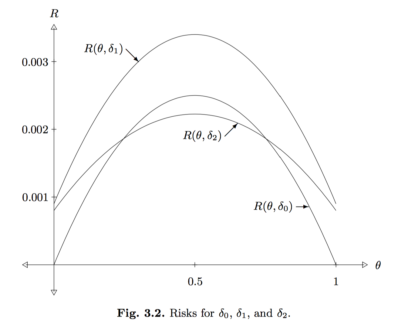
In the above, he uses a third estimator, \(\delta_1(X) = (X+3)/100\), and also, \(\delta_0(X) = X/100\) is the original estimator and \(\delta_2(X) = (X+3)/106\).

It is intuitive that \(\delta_1\) is a poor estimator of \(\theta\) because it adds 3 (i.e., like adding “three heads”) without doing anything else. In fact, we can rigorously say that \(\delta_1\) is dominated by both \(\delta_0\) and \(\delta_2\) because, throughout the entire support for \(\theta\), the risk associated with \(\delta_1\) is higher than the other estimators. The comparison between \(\delta_0\) and \(\delta_2\) is less straightforward; when the true \(\theta\) value is near \(1/2\), we’d prefer \(\delta_2\) for instance, but the reverse is true near 0 or 1.

To wrap up this discussion, I’d like to connect the concept of risk with the bias-variance tradeoff, which introduces two key concepts to know (i.e., bias and variance). The bias of an estimator \(\delta(X)\) is defined as \(b(\theta, \delta) = \mathbb{E}[\delta(X)] - \theta\), where here we write \(\theta\) instead of \(g(\theta)\) for simplicity. The variance is simply \({\rm Var}(\delta(X))\) and usually involves computations involving the variance of \(X\) directly.

Problem 1 in Chapter 3 of Keener introduces the very interesting fact that the risk of an arbitrary estimator \(\delta\) under squared error loss is \({\rm Var}(\delta(X)) + b^2(\theta, \delta)\), or more intuitively, \(V + B^2\). In fact, I earlier saw this result stated in one of the two papers I discussed in my post on minibatch MCMC methods. In Section 3 of Austerity in MCMC Land: Cutting the Metropolis-Hastings Budget, the paper states without proof:

The risk can be defined as the mean squared error in \(\hat{I}\), i.e. \(R = \mathbb{E}[(I - \hat{I})]\), where the expectation is taken over multiple simulations of the Markov chain. It is easy to show that the risk can be decomposed as \(R = B^2 + V\), where \(B\) is the bias and \(V\) is the variance.

The first thing I do when I see rules like these is to try an example. Let’s test this out with one of our earlier estimators, \(\delta_0(X) = X/100\). Note that this estimator is unbiased, which means the bias is zero, so we simply need to compute the variance:

and this precisely matches the risk from earlier!

To prove that the risk can be decomposed this way in general, we can do the following (using \(\theta\) in place of \(g(\theta)\) and \(\delta\) in place of \(\delta(X)\) to simplify notation):

as desired! In the above, we expanded the terms (also by cleverly adding zero), applied linearity of expectation, applied the fact that \(\mathbb{E}[\mathbb{E}[\delta(X)]]\) is just \(\mathbb{E}[\delta(X)]\), and also used that \(\mathbb{E}[\delta - \mathbb{E}[\delta]] = 0\).

I was recently reading Stephen Tu’s blog and stumbled upon his matrix inverse equality post which brough back some memories. Here’s the equality: let \(X\) be an \(n \times d\) matrix, let \(\lambda > 0\), and let \(I_k\) represent the \(k \times k\) identity matrix. Then

Note that both sides are left-multipled by \(X\), so for the purposes of checking equality, there’s no need to have it there, so instead consider

I was asked to prove this as part of a homework assignment in my CS 281A class with Professor Ben Recht a while back. Stephen Tu already has an excellent proof based on Singular Value Decomposition, but I’d like to present an alternative proof that seems even simpler to me. I also want to explain why this equality is important.

First, start with \(\lambda X^T = \lambda X^T\). Then left-multiply the left hand side (LHS) by \(I_d\) and right-multiply the right hand side (RHS) by \(I_n\) to obtain

Note that this doesn’t change the equality, because multiplying a matrix with the identity will not change it, regardless of the multiplication ordering. As a sanity check, the LHS is \((d \times d)\times (d \times n)\) and the RHS is \((d\times n)\times (n\times n)\) and both result in a \((d \times n)\)-dimensional matrix so the dimensions match up. Next, add \(X^TXX^T\) to both sides and get

We now “distribute out” an \(X^T\), though the particular \(X^T\) to use is different on both sides. We obtain

Next, left-multiply both sides by \((X^TX + \lambda I_d)^{-1}\) and right-multiply both sides by \((XX^T + \lambda I_n)^{-1}\):

Thus proving the identity.

Now, you can leave it like that and in some cases you’ll be OK. But strictly speaking, you should show that the two inverses above actually exist before using them. When I was writing up this for my homework, I said “the problem implies the inverses exist” because the inverse was already written in the problem statement. In retrospect, however, that was a mistake. Fortunately, the TA didn’t take off any points, though he marked “No, but w/e …”

To make things extra clear, we now show that the inverses exist. Consider \((X^TX + \lambda I_d)\). We claim its inverse exist because it is positive definite (and all positive definite matrices are invertible). This is straightforward because for any nonzero \(z \in \mathbb{R}^d\), we have

where we use the standard \(w^Tw = \|w\|_2^2\) trick, which is everywhere in machine learning and optimization. If you don’t believe me, take EE 227B as I did and you’ll never be able to forget it. By the way, the above shows why we needed \(\lambda > 0\), because \(\|Xz\|_2^2\) is not necessarily greater than zero; it could be zero! This is because \(X^TX\) could be positive semi-definite, but not positive definite.

A similar proof applies for the other inverse, which uses \(\|X^Ty\|_2^2\) for \(y \in \mathbb{R}^n\).

Having proved the equality, why do we care about it? The reason has to do with ridge regression and duality. The problem formulation for ridge regression is

where \(y\) is the \(n\)-dimensional vector of targets and \(\lambda > 0\). Taking the gradient we get

Setting to zero, we find \(w^*\) as

Gee, does this formulation of \(w^*\) look familiar? Yep! The above is one way of finding \(w^*\), but another way is by invoking the equality to get what is known as the dual form of \(w^*\):

Why do we like this new perspective? First, like any dual solution, it provides us with an alternative method if the “other” way (technically called the primal solution) is harder to compute. In this case, however, I don’t think that’s the main reason why (because this is fairly straightforward either way). I think we like this representation because \(w^*\) is a linear combination of the rows of \(X\), with coefficients specified by the vector \(\alpha^* \in \mathbb{R}^n\)! The rows of \(X\) are the elements in our data \(\{x_i\}_{i=1}^n\), so this gives the intuitive interpretation of the optimal solution being some combination of the data elements.

Suppose there are two people talking in sign language. What should you do when you have to walk in between them in order to reach your destination? If the people were talking verbally (say, in English), you would walk through the two without hesitation.

But does sign language cause the etiquette to be different?

I thought about this recently when I was attending a recent tour. As part of it, the attendees listened to a few talks in an auditorium. Since I had a sign language interpreter, I naturally sat in the front corner seat of the room. Fortunately, I didn’t play my usual role of the “human repellent.” Despite there being lots of empty seats, some of the other people actually sat next to me instead of being afraid of the sign language and consequently sitting as far away from me as possible. (I hope that’s the reason why people generally don’t sit next to me …)

I didn’t know anyone else in the tour, so during breaks within the talks, I would strike up some conversations with the sign language interpreter. At the same time, a lot of the other attendees needed to get up and walk to the back of the auditorium, presumably to fetch a new batch of Starbucks coffee. But this meant that many had to cut through me and the sign language interpreter. Throughout the tour, I noticed two classes of people:

1. Those who walked through our conversation quickly and without hesitation.

2. Those who paused and nervously glanced at me and the interpreter, wondering about what to do.

I’m here to reassure you that (1) is much better than (2). If you need to walk between us to go somewhere, please do it (quickly).

I think most people who engage in (2) are those who do not have much experience with sign language and “deafness” more generally, so their reaction is certainly understandable (and a sign of politeness, I might add). When this situation happens, usually the sign language interpreter will quickly motion for the person to walk through, and then he or she will do a little sprint and then continue walking.

Perhaps people are worried about some unknown rules of sign language etiquette? If so, don’t worry: I don’t find walking between us to be rude at all, and I have yet to meet anyone who gets bothered by this. It doesn’t interfere with our conversation that much, because (just like in English audio) if a second of the conversation (or audio) gets cut, we can usually fill in the details by means of continuity, which comes with experience using the language.

If there’s a group of people who have to walk between us, then it’s a different story. When that happens, we have to pause the sign language until everyone gets through, but that’s understandable; we don’t want to be jerks and force everyone to take a far more roundabout route.

To state the obvious, though: if there’s a way to get to your destination without cutting through our conversation, you should consider that alternative route, but if that would require squeezing between a twelve-inch gap between the wall of the auditorium and the back of my interpreter’s chair and making yourself look silly in the process, please don’t do it. If you would walk between us without hesitation if we were talking in English, then you can safely walk in between a sign language conversation. That doesn’t mean walk, then stop, examine your clothes, fiddle around, and so forth. If you take more than a second, you’ll annoy us. Just act normally, please. That goes for a lot of other things related to deafness that I’ve experienced in my life.

More games are jumping on the AI bandwagon.

We saw IBM’s Deep Blue, which beat chess Grandmaster Gary Kasparov in 1997. Then in 2013, we saw DeepMind’s AI agents¹ achieve human-level performance on many classic Atari 2600 games. Then earlier this year, we saw DeepMind’s next product, AlphaGo, beat Lee Sodol in a widely publicized Go match. You can view the details on DeepMind’s AlphaGo website, which also has the corresponding Nature paper. I have not read it yet (it’s on my TODO-list), but I read and considerably enjoyed their other Nature paper (from 2015) about Atari 2600 games.

Yet it looks like we are not done with AI and games. The news is out that Microsoft Research has made Project Malamo open source! It allows people to use the popular sandbox game Minecraft for AI research. Microsoft has been using it for a few months, as evident by this earlier article, but I only found out about Project Malamo after it became open source. Ironically, I didn’t find this by browsing Microsoft’s website — I found it on the Minecraft forum website.

Their overall goal is stated as follows:

[…] five computer scientists are spending their days trying to get a Minecraft character to climb a hill.

That may seem like a pretty simple job for some of the brightest minds in the field, until you consider this: The team is trying to train an artificial intelligence agent to learn how to do things like climb to the highest point in the virtual world, using the same types of resources a human has when she learns a new task.

That means that the agent starts out knowing nothing at all about its environment or even what it is supposed to accomplish. It needs to understand its surroundings and figure out what’s important – going uphill – and what isn’t, such as whether it’s light or dark. It needs to endure a lot of trial and error, including regularly falling into rivers and lava pits. And it needs to understand – via incremental rewards – when it has achieved all or part of its goal.

Stated succinctly, they want to train the player to get to higher ground in Minecraft, without having to explicitly code that concept. One can formulate this as a reinforcement learning problem using some form of a Markov Decision Process (you can view my earlier article on MDPs here). As in the case for DeepMind’s work, the researchers of Project Malamo want to accomplish this while only relying on information that a human can see. That is, they want the agent to learn like a human would. This is definitely going to be a challenging problem. Minecraft is one of the most open-ended games ever, and even humans are often unsure of what their objectives are when playing. I’ve had people tell me, “what’s the point of Minecraft?”

The researchers are constraining their focus to “moving uphill”, which helps to narrow down the problem. That still results in a very broad game, and is unlike previous work using Chess, Go, and Atari 2600 games, which have clearer goals for the player. I will be particularly interested in seeing how researchers will compare their results. How do we evaluate the quality of agents? I am also curious about what role deep learning will play in this research.

On a final note, if they want an AI enthusiast who is also a Minecraft enthusiast to serve as a contributor … my contact information is on the “About” page of this website. Unfortunately, I have not played Minecraft in months (maybe a year?!?) and my guess is that a disproportionate share of computer scientists are also Minecraft players.

I took a break from paper reviewing to be in Washington DC for a few days. This marked my first time being in the city, and it’s been a pleasure to tour arguably the most important one of our country. My visit coincided with the July 4 weekend, so there was a lot of patriotism on display. Among my itinerary in Washington DC was Capitol Hill and the Smithsonian National Air and Space Museum. Both are government-controlled entities, which means that admission is free (because we pay for it with our taxes¹) and that they are expected to provide reasonable accommodations for people with disabilities.

Just to be clear, I don’t want to suggest that the private sector doesn’t do a good job providing accommodations. I do, however, believe that government agencies might be slightly, slightly more sensitive for the need to provide disability-related accommodations. After all, wouldn’t it be an embarrassment if they failed to follow the Americans with Disabilities Act?

Not having done much planning in advance (thank you, paper reviewing!) I didn’t know what to expect with regards to accommodations. Fortunately, my Capitol Hill visit turned out quite well. Despite not having a reservation, I was able to participate in a guided tour of the building. This was split in two parts. The first was a brief introductory video which described our nation’s remarkable history in 10-15 minutes. Fortunately, it had open captioning, so I was able to understand it.

The second part was the actual building tour. There were so many people that the guides split us up into five groups, each with our own guide. What was interesting, though, was that we were all provided headsets so that we could hear our tour guide speaking in his microphone (and only our tour guide, not the others). This worked out well when we were in crowded areas with several tour guides talking at once. For me, of course, I wouldn’t have benefited much from the headsets. Fortunately, after inquiring, I got a T-Coil necklace, and wow, that really amplified my guide’s voice! It was even louder than what I’m used to with FM systems, and on top of it all, there was no static. As a result, I understood most of what my guide said throughout the tour. Speaking of the actual tour, it was a nice experience looking inside Capitol Hill; we passed by Speaker Paul Ryan’s office, though we obviously didn’t see the Speaker himself. We didn’t get to explore much of the building, unfortunately, and there is still substantial construction going on, obscuring much of the inner Capitol Hill dome. Perhaps later I can try and get a better tour by submitting my name in the lottery for the tours arranged by the California Representatives or Senators? Nonetheless, it was still a good experience for me and I was happy with the tour and the accommodations.

I had a different experience at the Smithsonian Museum. After touring some of the ground floor exhibits, I paid a ticket for one of their “featured films”. I first asked for the standard (non-IMAX) film that was closest to starting, but after I asked, the cashier told me it did not have captions, and she recommended I instead watch A Beautiful Planet, offered in IMAX. Once the doors opened to enter the theater, I lined up with everyone to take our 3D glasses. I found my way into a good seat in the center of the auditorium, and … there were no captions. IMAX films are quite loud, but even so, I could not make out the conversations among the astronauts in the film. I actually fell asleep about ten minutes into it out of boredom, and woke up at the end of the film. I was a bit disappointed that an IMAX film causes me to nap rather than watch a movie (and no, I didn’t even turn off my hearing aids). I wonder: should I have asked for more details on the captioning? I don’t recall the exact words I uttered, but it’s true that I could always have been more specific with my wording. Or was I supposed to get different 3D glasses, kind of like how I got a different kind of “headset” for the tour guide? I wouldn’t be surprised if they had closed captioning glasses. Or now that I think about it, did I simply mishear the person who I asked about this?

Lesson learned: I need to ask more questions, and to plan ahead for these once-in-a-few-years visits.

This year, I volunteered to be a NIPS reviewer, since I want to get the experience of reviewing academic papers. It was pretty easy to volunteer: for every paper submitted to NIPS, they asked that at least one of the authors offer to be a reviewer, and preferably not someone who’s already on their list of known reviewers. I’m clearly not among that elite crowd, and I wanted to review anyway, so it was an easy choice for me.

This year, NIPS had around 2500 (!) paper submissions, according to the number I saw in the Conference Management Toolkit website, which is what NIPS uses to manage paper submissions and reviews. I think the exact number I saw was roughly 2450-ish, but it’s worth noting that papers with authors who match my conflict of interest domains (especially “berkeley.edu”) wouldn’t appear on this list. When I was submitting my paper bids for reviewing purposes, I couldn’t find the paper I submitted (fortunately!).

For obvious reasons, I can’t divulge too much about the papers I’m reviewing. But I can probably safely say this: I got assigned four papers to review in the span of roughly a month (from June 17 to July 17). So I’m reviewing right now, and decided to write this blog post during one of my breaks. Now that I’ve read all my assigned papers and have more-or-less come up with a very high-level draft conclusion about them, here are four thoughts:

1. Unfortunately, I’m probably deeply qualified to review … none of the four papers. For two of the papers, I understand much of the main ideas, but I still lack intricate knowledge of the math and algorithms they use, and about the most prevalent related work. For two other papers, I’m close to being lost on them. Therefore, I have made this a rule: for each paper, I will allow myself to read one extra reference for background information. One. So effectively, my reading load for this cycle is eight papers, four to be read in-depth and four to be read semi-in-depth. This raises my curiosity: how do people actually carefully review papers? The vast majority of NIPS papers are extraordinarily specialized and technical, and many still have proofs in appendices. I don’t see how it is humanly possible for me to verify the proofs and make sure the math lines up correctly, especially with an internship that already takes up about 50 hours a week. It can take hours just to verify one simple line of equations in a paper, which might require looking through a previous paper reference, checking Wikipedia for additional background information, and then marking down an annoying typo that got me confused. Can an experienced NIPS reviewer please tell me how he or she reviews papers?

2. Fortunately, the previous thought might not matter because, despite not having gone through all the technical material so far (I’ve only been reviewing a week!) I feel like I can more or less tell how I feel about the papers. For instance, the amount of formalism and “cleanliness” of the paper gives a good clue about its quality. If the paper is rife with typos and sloppy LaTeX, or if the figures look spectacularly low-quality, that’s just asking for a rejection. (Come on, with matplotlib embedded in Jupyter notebooks, people should be able to produce acceptable figures.) Note that by this, I’m excluding language issues that might arise due to non-native English speakers writing the paper. It’s not fair to them.

3. It’s nice reviewing papers without knowing the identity of the authors. NIPS is double blind, which I believe to be a good thing, and I say this as someone who would probably benefit from an open reviewing process. I don’t want to think about the authors’ identities. I have not actively searched so I’m still in the dark about this for all four of my papers. As a reviewer, I like my identity being protected, so I’m reconsidering my earlier thought about making some of the reviews public (sadly, if this were politics, I’d be accused of “waffling”). Unfortunately, for one of my papers, I have a good feeling about who at least one of the authors is based on previous research, despite how I haven’t been in this field very long (and some would argue, have never been in this field). In addition, two of my other papers have a previous reference which is obviously similar to the current work, and since I ended up using those papers as my “background reference” material and seeing practically word-for-word similarities … author similarities follow. I’ll keep my guesses in mind and then see how they turn out later in August.

4. Despite my internship, I would bet I have more time on my hands than most faculty for reviewing, because I have fewer competing priorities and because I would be assigned fewer papers (hopefully … did I?). Thus, I will try to write some really detailed suggestions or at the very least, thought-provoking comments/questions, and I think the authors would appreciate that even if their papers don’t get accepted. At all costs, I am not going to be writing those dreaded three line reviews that contribute nothing. Sadly, I frequently see these online at the NIPS proceedings, which makes reviews public for accepted papers. As a result, this period from mid-June to mid-July is going to be super busy for me, since I am doing all my reviewing in nights and weekends. I am really trying to make sure my reviews are helpful.

That’s all for now — I need to get back to reviewing.

I have recently been working on minibatch Markov chain Monte Carlo (MCMC) methods for Bayesian posterior inference. In this post, I’d like to give a brief summary of what that means and mention two ICML papers (from 2011 and 2014) that have substantially influenced my thinking.

When we say we do “MCMC for Bayesian posterior inference,” what this typically means is that we have some dataset \(\{x_1,x_2,\ldots,x_N\}\) and a parameter of interest \(\theta \in \mathbb{R}^K\) for some \(K \ge 1\). The posterior distribution \(f(\theta)\) we wish to estimate (via sampling) is

You’ll notice that we assume the data is conditionally independent given the parameter. In many cases, this is unrealistic, but most of the literature assumes this for simplicity.

After initializing \(\theta_0\), the procedure for sampling the posterior on step \(t+1\) is:

• Draw a candidate \(\theta'\)
• Compute the acceptance probability (note that the denominators of \(f\) cancel out):

• Draw \(u \sim {\rm Unif}[0,1]\), and accept if \(u < P_a\). This means setting \(\theta_{t+1} = \theta'\). Otherwise, we set \(\theta_{t+1} = \theta_t\) and repeat this loop. This tripped me up earlier. Just to be clear, we generate a sample \(\theta\) every iteration, even if it is a repeat of the previous one.

This satisfies “detailed balance,” which roughly speaking, means that if one samples long enough, one will arrive at a stationary distribution matching the posterior, though a burn-in period and/or only using samples at regular intervals is often done in practice. The resulting collection of (correlated!) samples \(\{\theta_1, \theta_2, \ldots, \theta_T\}\) for large \(T\) can be used to compute the value of \(p(\theta \mid x_1,\ldots,x_N)\). Let’s consider a very simple example. Say \(\theta\) can take on three values: \(A\), \(B\), and \(C\). If our sampled set is \(\{A,B,B,C\}\), then since \(B\) appears two times out of four, we have \(p(\theta = B \mid x_1,\ldots,x_N) = 2/4\). The other two probabilities would naturally have \(1/4\) each according to the samples.

One issue with the standard procedure above is that in today’s big data world with \(N\) on the order of billions, it is ridiculously expensive to compute \(P_a\) because that involves determining all \(N\) of the likelihood factors. Remember, this has to be done every iteration! Doing all this just to get one bit of data (whether to accept or not) is not a good tradeoff. Hence, there has been substantial research on how to perform minibatch MCMC on large datasets. In this case, rather than use all \(N\) data points, we just use a subset \(n \ll N\) of points each iteration. This approximates the target distribution. The downside? It no longer satisfies detailed balance. (I don’t know the details on why, and it probably involves some complicated convergence studies, but I am willing to believe it.)

Just to be clear, we are focusing on getting a distribution, not a point estimate. That’s the whole purpose of Bayesian estimation! A distribution means we need a full probability function that sums to one and is non-negative; if \(\theta\) is one or two dimensional, we can easily plot the posterior estimate (I provide an example of this later in this post). A point estimate means finding one value of \(\theta^*\), usually the “best”, which we commonly express as the maximum likelihood estimate \(\theta^* = \theta_{\rm MLE}\).

All right, now let’s briefly discuss two papers that tackle the problem of minibatch MCMC.

Bayesian Learning via Stochastic Gradient Langevin Dynamics

This paper appeared in ICML 2011 and proposes using minibatch update methods for Bayesian posterior inference, with a concept known as Langevin Dynamics to inject the correct amount of noise into parameter updates so that the set of sampled parameters converges to the posterior, and not just a mode. To make the distinction clear, let’s see how we can use minibatch updates to converge to a mode — more specifically, the maximum a posteriori estimate. The function \(f\) we are trying to optimize is listed above. So … we just use stochastic gradient ascent! (We are ascending, not descending, because \(f\) is a posterior probability, and we want to make its values higher.) This means the update rule is as follows: \(\theta_{t+1} = \theta_t + \alpha_t \nabla f(\theta_t)\). Plugging in \(f\) above, we get

where \(\epsilon_t\) is a sequence of step sizes.

The above is a stochastic gradient ascent update because we use \(n \ll N\) terms to approximate the gradient value, which is why I inserted an approximation symbol (\(\approx\)) in the underbrace. Because we only use \(n\) terms, however, we must multiply the summation by \(N/n\) to rescale the value appropriately. Intuitively, all those terms in that summation are negative since they’re log probabilities. If we use \(n\) instead of \(N\) terms, that summation is strictly smaller in absolute value. So we must rescale to make the value on the same order of magnitude. Another way of putting it is that the subsampled sum will be an unbiased estimator of the full-batch quantity.

What’s the problem with the above for Bayesian posterior inference? It doesn’t actually do Bayesian posterior inference. The above will mean \(\theta\) converges to a single value. We instead want a distribution. So what can we do? We can use Langevin Dynamics, meaning that (for the full batch case) our updates are:

A couple of things are worth noting:

• We use all \(N\) terms in the summation, so the gradient is in fact exact.
• The injected noise \(\eta_t\) means the \(\theta_{t}\) values will “bounce around” to approximate a distribution and not converge to a single point.
• The \(\epsilon\) is now constant instead of decreasing, and is balanced so that the variance of the injected noise matches that of the posterior.
• We use \(x_i\) instead of \(x_{ti}\) as we did earlier. The only difference is that the \(t\) indicates the randomness in the minibatch. It does not mean that \(x_{ti}\) is one scalar element of a vector. In other words, both \(x_i\) and \(x_{ti}\) are in \(\mathbb{R}^k\) for some \(k\).

For simplicity, the above assumes that \(\eta_t \in \mathbb{R}\). In the general case, these should be multivariate Gaussians, with covariance \(\epsilon I\).

The problem with this, of course, is the need to use all \(N\) points. So let’s use \(n \ll N\) points, and we have the following update:

where now, we need \(\epsilon_t\) to vary and decrease towards zero. The reason for this is that as the step size goes to zero, the corresponding (expensive!) Metropolis-Hastings test has rejection rates that decrease to zero. Thus, we can omit the test to make the algorithm computationally cheap.

Fortunately, the authors show that despite how the noise goes to zero, the set of samples from SGLD will indeed converge to the correct posterior distribution, just as with “normal” (i.e., full-batch) Langevin Dynamics noise.

Austerity in MCMC Land: Cutting the Metropolis-Hastings Budget

This paper appeared in ICML 2014, and is also about minibatch MCMC. Here, instead of relying on simulating the physics of the system (as was the case with Stochastic Gradient Langevin Dynamics), they propose reformulating the standard MCMC method with the standard MH test into a sequential hypothesis test. To frame this, they take the log of both sides of the acceptance inequality:

In the first step we also dropped the initial “min” because if the “1” case applies, we will always accept. In the last step we divide both sides by \(N\). What is the purpose of this? The above is equivalent to the original MH test. But the right hand side depends on all \(N\) data points, so what happens if we compute the right hand side using \(n \ll N\) points?

This is the heart of their test. They start out by using a small fraction of the points and compute the right hand side. If the proposed \(\theta'\) element is so out of whack, then even with just \(n\) points, we should already know to reject it. (And a similar case holds if \(\theta'\) is really good.) If we cannot tell whether to accept or reject \(\theta'\) with some specified confidence threshold, then we increase the minibatch size and test again. Their acceptance test relies on the Central Limit Theorem and the Student-t distribution. The details are in the paper, but the main idea is straightforward: increasing the number of samples increases our certainty as to whether we accept or reject, and we can generally make these decisions with far fewer than \(N\) samples.

What’s the downside of their algorithm? In the worst case, we might need the entire data in one iteration. This may or may not be a problem, depending on the particular circumstances.

Their philosophy runs deeper than what the above says. Here’s a key quote:

We advocate MCMC algorithms with a “bias-knob”, allowing one to dial down the bias at a rate the optimally balances error due to bias and variance.

One other algorithm that adheres to this strategy? Stochastic Gradient Langevin Dynamics! (Not coincidentally, Professor Max Welling is a co-author on both papers.) Side note: the reason why SGLD is biased is because it omits the Metropolis-Hastings test. The reason why this algorithm (Adaptive Sampling) is biased is because it makes decisions based on a fraction of the data. So both are biased, but for slightly different reasons.

Putting it All Together: A Code Example

In order to better understand the two papers described above, I wrote some Python code to run SGLD and adaptive sampling. I also implemented the standard (full-batch) MCMC method for a baseline.

I tested using the experiment in Section 5.1 of the SGLD paper. The parameter is 2-D, \(\theta = (\theta_1,\theta_2)\), and the parameter/data generation process is

and

I’ve pasted all my Python code here. If you put this together in a Jupyter notebook, it should work correctly. If your time is limited, feel free to skip the code and go straight to the output. The code is here mainly for the benefit of current and future researchers who might want a direct implementation of the above algorithms.

The first part of my code imports the necessary libraries and generates the data according to my interpretation of their problem. I am generating 500 points here, whereas the SGLD paper only used 100 points.

# Import necessary libraries
import numpy as np
import matplotlib.pyplot as plt
%matplotlib inline
from scipy.stats import t

# Generate the data according to Section 5.1 of "Bayesian Learning via SGLD."
N = 500 # The number of data points; we reference this frequently later.
sigma1_sq = 10
sigma2_sq = 1
sigmax_sq = 2
theta1 = 0
theta2 = 1

# Generate the data X. The np.random.normal(...) requires STD (not VAR).
X = np.zeros(N)
for i in xrange(N):
    u = np.random.random()
    if (u < 0.5):
        X[i] = np.random.normal(theta1, np.sqrt(sigmax_sq))
    else:
        X[i] = np.random.normal(theta1+theta2, np.sqrt(sigmax_sq))

Next, I define a bunch of functions that I will need for the future. The most important one is the log_f function, which returns the log of the posterior. (Implementing this correctly requires filling in some missing mathematical details that follow from the formulation of multivariate Gaussian densities.)

def log_f(theta, X):
    """
    The function 'f' is the posterior:
    
        f(\theta) \propto p(\theta) * \prod_{i=1}^N p(x_i | \theta)
    
    This method returns the *log* of f(\theta), for obvious reasons.
    X is assumed to be of shape (n,) so we reshape it into (n,1) for vectorization.
    We use [0,0] since we get a float in two lists, [[x]], so calling [0,0] gets x.
    """
    scale = N / float(len(X))
    
    inverse_covariance = np.array([[0.1,0],[0,1]])
    prior_constant = 1.0 / (2*np.pi*np.sqrt(10))
    prior = np.log(prior_constant) - 0.5*(theta.T).dot(inverse_covariance).dot(theta)
    
    X_all = X.reshape((len(X),1))
    ll_constant = (1.0 / (4*np.sqrt(np.pi)))
    L = ll_constant * (np.exp(-0.25*(X_all-theta[0])**2) + np.exp(-0.25*(X_all-(theta[0]+theta[1]))**2))
    log_likelihood = np.sum(np.log(L)) * scale
    
    assert not np.isnan(prior + log_likelihood)
    return (prior + log_likelihood)[0,0]
    
    
def grad_f(theta, X):
    """ Computes gradient of log_f by finite differences. X is (usually) a mini-batch. """
    eps = 0.00001
    base1 = np.array([[eps],[0]])
    base2 = np.array([[0],[eps]])
    term1 = log_f(theta+base1, X) - log_f(theta-base1, X)
    term2 = log_f(theta+base2, X) - log_f(theta-base2, X)
    return np.array([[term1],[term2]])/(2*eps)
    
 
def get_delta(theta_c, theta_p, X):
    """
    Compute the delta term, so we use min{1, exp(\Delta')} for standard MCMC.
    
    theta_c is the *current* theta that we may "leave" (old theta)
    theta_p is the *proposed* theta that we might accept (new theta)
    """
    loss_old = log_f(theta_c, X)
    loss_new = log_f(theta_p, X)
    assert not np.isnan(loss_new - loss_old)
    return loss_new - loss_old


def get_noise(eps):
    """ Returns a 2-D multivariate normal vector with covariance matrix = diag(eps,eps). """
    return (np.random.multivariate_normal(np.array([0,0]), eps*np.eye(2))).reshape((2,1))


def log_f_prior(theta):
    """
    Returns log p(\theta), the prior. Remember, it's returning LOGS. Don't take logs again! 
    This is only used for the adaptive sampling method's hypothesis testing.
    """
    cov_inv = np.array([[0.1,0],[0,1]])
    return np.log(1.0/(2*np.pi*np.sqrt(10))) - 0.5*(theta.T).dot(cov_inv).dot(theta)
        
        
def approximate_mh_test(theta_c, theta_p, m1, X, mu_0, eps_tolerance):
    """
    Implements the adaptive sampling method. Each time we call this, we shuffle the data.
    
    theta_c is the current \theta
    theta_p is the proposed \theta
    m1 is the starting minibatch size
    X is the full data matrix
    mu_0 is equation 2 from "Cutting the MH" paper, pre-computed
    eps_tolerance is for deciding whether delta is small enough
    
    Returns ('accept', 'size'), where 'accept' is a boolean to indicate if we accept or not,
        while 'size' is the size of the mini-batch we sampled (generally a multiple of m).
    """
    
    accept = False
    done = False
    first_iteration = True
    n = 0
    m2 = m1 # We'll increment by the same amount as 'm1', the starting size.
    
    # Shuffle at beginning so we can do X_mini = X[:n]
    index = np.random.permutation(N)
    X = X[index]

    while not done:
        
        # Draw mini-batch without replacement, but keep using same indices we've used.
        # Note that we can have a special case for the first minibatch.
        if first_iteration:
            size = np.min([m1, N])
            first_iteration = False
        else:
            size = np.min([m2, N-n])
        n = n + size
        X_mini = (X[:n]).reshape((n,1)) # To enable broadcasting
        
        # Now compute ell_bar and ell_bar_squared, which rely on the data.
        numerator   = np.exp( -0.25*(X_mini-theta_p[0])**2 ) + np.exp( -0.25*(X_mini-(theta_p[0]+theta_p[1]))**2 )
        denominator = np.exp( -0.25*(X_mini-theta_c[0])**2 ) + np.exp( -0.25*(X_mini-(theta_c[0]+theta_c[1]))**2 )
        log_terms = np.log( numerator / denominator )
        ell_bar = (1.0/n) * np.sum(log_terms)
        ell_bar_squared = (1.0/n) * np.sum(log_terms**2) # Squaring individual terms!
        
        # Let's just be safe and check for NaNs.
        assert not np.isnan(np.sum(numerator))
        assert not np.isnan(np.sum(denominator))
        assert not np.isnan(ell_bar)
        assert not np.isnan(ell_bar_squared)
        
        # Now we have the information needed to compute s_l, s, |t|, and delta.
        # Note that if n == N, we can exit since we know delta should be 0. We have all the data.
        if (n == N):
            delta = 0
        else:           
            s_l = np.sqrt((ell_bar_squared - (ell_bar**2)) * (float(n)/(n-1)))
            s = (s_l / np.sqrt(n)) * np.sqrt(1 - (float(n-1)/(N-1)))
            test_statistic = np.abs((ell_bar - mu_0) / s)
            delta = 1 - t.cdf(test_statistic, n-1)
            assert not np.isnan(delta)
            assert not np.isnan(s)
        
        # Finally, we can test if our hypothesis is good enough.
        if (delta < eps_tolerance):
            if (ell_bar > mu_0):
                accept = True
            done = True
  
    return (accept,n)

Next, I run three methods to estimate the posterior: standard full-batch MCMC, Stochastic Gradient Langevin Dynamics, and the Adaptive Sampling method. Code comments clearly separate and indicate these methods in the following code section. Note the following:

• The standard MCMC and Adaptive Sampling methods use a random walk proposal.
• I used 10000 samples for the methods, except that for SGLD, I found that I needed to increase the number of samples (here it’s 30000) since the algorithm occasionally got stuck at a mode.
• The minibatch size for SGLD is 30, and for the Adaptive Sampling method, it starts at 10 (and can increase by 10 up to 500).

############################
# STANDARD FULL-BATCH MCMC #
############################
num_passes = 10000
rw_eps = 0.02
theta = np.array([[0.5],[0]])
all_1 = theta # Our vector of theta values

for T in range(1,num_passes):
        
    # Standard MH test. Note that it's just min{1, exp(\Delta')}.
    theta_new = theta + get_noise(rw_eps)        
    delta_real = get_delta(theta, theta_new, X)
    test = np.min([1, np.exp(delta_real)])
    u = np.random.random()
    
    # Perform test of acceptance. Even if we reject, we add current theta to all_1.
    if (u < test):
        theta = theta_new
    all_1 = np.concatenate((all_1,theta), axis=1)
        
print("\nDone with the standard minibatch MCMC test.\n")


#########################################
# STOCHASTIC GRADIENT LANGEVIN DYNAMICS #
#########################################
num_passes = 30000
theta = np.array([[0.5],[0]])
all_2 = theta
mb_size = 30

# a and b are based on parameter values similar to those from the SGLD paper.
a = 0.06
b = 30

for T in range(1,num_passes): 

    # Step size according to the SGLD paper.
    eps = a*((b + T) ** (-0.55))
    
    # Get a minibatch, then compute the gradient, then the corresponding \theta updates.
    X_mini = X[np.random.choice(N, mb_size, replace=False)]
    gradient = grad_f(theta, X_mini)
    theta = theta + (eps/2.0)*gradient + get_noise(eps)
    
    # Add theta to all_2 and repeat.
    assert not np.isnan(np.sum(theta))
    all_2 = np.concatenate((all_2,theta), axis=1)
    
print("\nDone with Stochastic Gradient Langevin Dymamics.\n")


############################
# ADAPTIVE SAMPLING METHOD #
############################
num_passes = 10000
rw_eps = 0.02
mb_size = 10
theta = np.array([[0],[1]])
all_3 = theta
tolerance = 0.025

for T in range(1,num_passes):
    
    # Let's deal with the Approx_MH test. This returns a boolean to accept (True) or not.
    # With a random walk proposal, the mu_0 does not depend on the likelihood information.
    theta_new = theta + get_noise(rw_eps)
    prior_old = log_f_prior(theta)
    prior_new = log_f_prior(theta_new)
    log_u = np.log(np.random.random())
    mu_0 = (1.0/N) * (log_u + prior_old - prior_new)    
    (do_we_accept, this_mb_size) = approximate_mh_test(theta, theta_new, mb_size, X, mu_0, tolerance)
    
    # Several checks, just to be safe.
    assert not np.isnan(prior_old)
    assert not np.isnan(prior_new)
    assert not np.isnan(log_u)
    assert not np.isnan(mu_0)
    assert this_mb_size >= mb_size
    
    # The usual acceptance test, and updating all_3.
    if do_we_accept:
        theta = theta_new
    all_3 = np.concatenate((all_3,theta), axis=1)
        
print("\nDone with the adaptive sampling method!\n")

With the sampled \(\theta\) values in all_1, all_2, and all_3, I can now plot them using my favorite Python library, matplotlib. I also create a contour plot of what the log posterior should really look like.

# Let's form the plot. This will be one figure with four sub-figures.
mymap2 = plt.get_cmap("Greys")
m_c2 = mymap2(400)
fig, axarr = plt.subplots(1,4, figsize=(16, 5))
(xlim1,xlim2) = (-1.5,2.5)
(ylim1,ylim2) = (-3,3)

# A contour plot of what the posterior really looks like.
axarr[0].set_title("Log Posterior Contour", size="xx-large")
K = 200
xlist = np.linspace(-1.5,2.5,num=K)
ylist = np.linspace(-3,3,num=K)
X_a,Y_a = np.meshgrid(xlist, ylist)
Z_a = np.zeros((K,K))
for i in range(K):
    for j in range(K):
        theta = np.array( [[X_a[i,j]],[Y_a[i,j]]] )
        Z_a[i,j] = log_f(theta, X)        
axarr[0].contour(X_a,Y_a,Z_a,300)

# The standard MCMC method
axarr[1].set_title("Standard MCMC", size="xx-large")
axarr[1].scatter(all_1[0], all_1[1], color = m_c2, alpha=0.15)
axarr[1].set_xlim([xlim1,xlim2])
axarr[1].set_ylim([ylim1,ylim2])

# Stochastic Gradient Langevin Dynamics
axarr[2].set_title("S.G.L.D. $(m=30)$", size="xx-large")
axarr[2].scatter(all_2[0], all_2[1], color = m_c2, alpha=0.15)
axarr[2].set_xlim([xlim1,xlim2])
axarr[2].set_ylim([ylim1,ylim2])

# The adaptive sampling method
axarr[3].set_title("Adaptive Sampling $(m=10)$", size="xx-large")
axarr[3].scatter(all_3[0], all_3[1], color = m_c2, alpha=0.15)
axarr[3].set_xlim([xlim1,xlim2])
axarr[3].set_ylim([ylim1,ylim2])

plt.tight_layout()
plt.savefig('blog_post_daniel.png', dpi=200)

By the way, it was only recently that I found out I could put LaTeX directly in matplotlib text. That’s pretty cool!

Here are the results in a scatter plot where darker spots indicate more points:

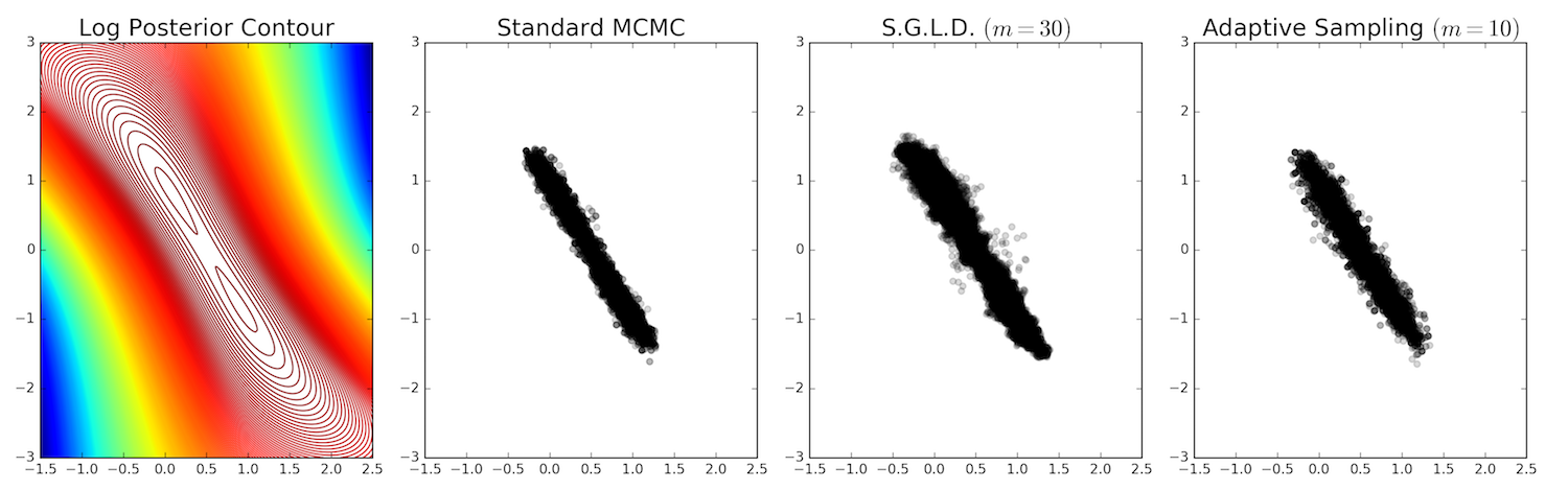
It looks like all three methods roughly obtain the same posterior form.

I just read Islam and the Future of Tolerance: A Dialogue, by renowned atheist Sam Harris and former jihadist-turned-liberal-activist Maajid Nawaz. I had this book on my radar for a while, and decided to read it yesterday in the wake of the tragic news of the recent Orlando shootings. My hope is to better understand what drives people to extremism and how we can reduce the probability of similar attacks from occurring.

I first found out about the book from browsing the website of Sam Harris, one of the four “New Atheists.” Harris and I see eye-to-eye on a number of issues. The most obvious one is that we are atheists. In addition, we both support LGBT rights, scientific reasoning, taxing billionaires, and we disapprove of the Iraq war. I do not claim to agree with everything he says, of course. Indeed, some of Harris’s statements have been controversial (as one would expect when dealing with religion). He actually felt compelled to write a blog post to respond to controversy.

As of this writing, Islam and the Future of Tolerance is Harris’ most recent book, but the interesting thing is that it’s actually a dialogue with Maajid Nawaz, listed as the book’s co-author. Nawaz has a remarkable personal story, which he describes in his 2013 autobiography Radical: My Journey Out Of Islamist Extremism. Nawaz was born in Britain, but after experiencing personal grievances (including racism), he joined the radical Islamist group Hizb ut-Tahrir. After an arrest in Egypt, he turned his life around by rejecting radical Islam. Today, he is of the world’s foremost liberal Muslims and a key challenger to extremism.

Islam and the Future of Tolerance is a conversation between Harris and Nawaz about Islam. Harris is skeptical that Nawaz can achieve the goal of reforming Islam. Harris, however, concedes that people like Nawaz — and not “infidels” like himself — are the ones who have to do the job. How can the faith reformation happen? What will be the future of Islam? That is the subject of their dialogue. Here are some of the highlights of their conversation, outlined according to the section:

• The Roots of Extremism. This is a short section where Nawaz provides an abbreviated version of his autobiography.

• The Scope of the Problem. Here’s the key takeaway: a primary issue with getting Muslims and non-Muslims to ally together is that the largest group of Muslims, which Harris and Nawaz call “religiously conservative Muslims”, do not wholeheartedly support contemporary liberal human rights. Thus, while those Muslims would be our allies against the Islamic State, they would also resist our efforts in promoting women’s rights, LGBT rights, etc.

• The Power of Belief. Harris asks Nawaz how he originally became radicalized. Was it due to “ordinary” grievances that might be corrected with more tolerance (e.g., turning to radical Islam due to racism from non-Muslims?), or due to deeper forces such as martyrdom? I have frequently wondered about this process because, as an atheist, I struggle to understand how something like religion (in its most extreme form) can systematically guide people towards terror, barbarianism, and destruction.

• The Betrayal of Liberalism. Both Harris and Nawaz slam liberals for their adherence to “political correctness.” (Donald Trump would be proud of them.) In the previous chapter, Harris rips liberal scholars who say that the West is to blame for the problems in Middle Eastern societies. Harris and Nawaz point out one unfortunate consequence of political correctness: that only right-wing bigots are accurately assessing jihadists nowadays.

• The Nature of Islam. Harris argues that most of our human rights progress in the last few centuries is despite the presence of religions such as Judaism, Christianity, and (especially) Islam. There are plenty of religious moderates, but Harris argues that these moderates somehow have to filter out the more dangerous parts of their scripture. Harris concludes that the purest interpretation of reading scripture — and therefore leaving out personal biases — would actually favor the Islamic State:

This is why the approach of a group like the Islamic State has a certain intellectual appeal (which, admittedly, sounds strange to say) because the most straightforward reading of scripture suggests that Allah advises jihadists to take sex slaves from among the conquered, decapitate their enemies, and so forth.

• Finding the Way Forward. Most of this section concerns the fatwa against the Islamic State. Harris and Nawaz, while recognizing that a fatwa is better than no fatwa, have reservations because it belies the true issues with Islamic tolerance. Near the end, Harris and Nawaz talk about the heavily American phenomenon of “being at war with Islam.” Harris admits that he may have played a role in assisting that culture, and Nawaz argues that President Obama must start naming the enemy radical Islam (I believe Nawaz is correct on this, but I also believe too much has been made out of this).

Despite the book’s brevity, I feel like both men were able to make good points. The conversation as a whole, while certainly not being a substitute for a more rigorous study of the role of religion in history, provides some interesting highlights. I learned about several historical events and spent some time browsing the corresponding Wikipedia pages to learn more.

One of my biggest takeaways from the book is that I doubt if liberals are effectively handling the problem of radical Islam. Harris and Nawaz, while both being liberals (in the sense that they would vote Democratic in the United States), would argue that liberals are not doing a good job. But they would also have that opinion of the conservative response.

But there’s something more important I need to mention. I think this conversation is useful because it shows how how people with different religious beliefs can come together and have a friendly, reasonable discussion without ripping each other’s throats. Nawaz is not that religious, but we need to have a starting point for a honest conversations with Muslims, and this dialogue serves that role effectively. In the wake of the Orlando shootings, these conversations give me hope that humanity will grow more peaceful and more tolerant in the coming years. Having an open mind is incredibly important. As Nawaz concludes:

Allow me to to take this opportunity to also thank you, Sam. It isn’t easy for anyone to reach across divides — real or imagined — and try to hold a sensible dialogue amid so much background noise and confusion. You will no doubt be censured by some Islam critics for not insisting that I am in fact a closet jihadist, just as I will be criticized by many Muslims for having this conversation with you.

Thanks to Sam Harris and Maajid Nawaz for having this conversation.