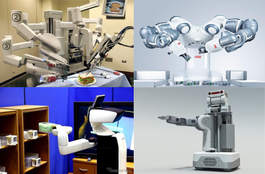Clockwise, starting from top left: the Da Vinci, the ABB YuMi, the PR2, and the Toyota HSR.

I now have several months of research experience in robotics. I am familiar with the following four robots, roughly in descending order of my knowledge of them:

• Da Vinci. Price: 2,000,000 USD (!!!). I’m not sure how much of the full set I use, though — I only use two of the arms, and the components might be cheaper versions. After all, even for well-funded Berkeley robotics labs, paying 2 million USD for a robot is impractical. Smaller hospitals also cannot afford the full Da Vinci.
• Toyota Human Support Robot (HSR). Price: ???. Oddly, I can’t find a price! In fact, I’m not even sure where to buy it.
• ABB YuMi. Price: 40,000 USD. At least this one is on the “cheap” end … I think?
• Personal Robot 2 (PR2), from Willow Garage¹. Price: 280,000 USD. Yikes! And that’s the open source version – the raw sticker cost started as 400,000 USD when it was released in 2010. Given that Willow Garage no longer exists, I’m not sure if it’s possible to buy a PR2.

I have sadly never touched or worked with the YuMi and the PR2, though I’ve manipulated the Da Vinci on a regular basis. The one-sentence summary: it’s a surgical robotics system which is currently the only such system approved by the U.S. Food and Drug Administration.

This is interesting. Now let’s switch to another topic: suppose you talk to a layperson about working in robotics. One typical, half-serious conversation involves this question: when will your robots take over the world?

I would respond by pointing out the obvious restrictions placed on the Da Vinci. It’s fixed to a base, with arms that perform a strictly limited set of surgery-related functions. So … it can’t really “join forces” with other Da Vincis and somehow navigate the real world.

But perhaps, your conversationalist argues, that we can take the arms of the Da Vinci and integrate them to a mobile robot (e.g. the Toyota HSR). If the Da Vinci works in surgical applications, then it must logically be very nimble-fingered². Think of the things it can do! It can pick locks, use car keys, redirect electric wires, and so forth.

Alas, from my experience, it’s difficult to even get the robot arms to go where I want to them to go. To make this more concrete, suppose we’re looking at an image of a flat surgical platform through the Da Vinci camera mounted above. When we look at the image, we can visually identify the area where we want the arm (or more precisely, the “end effectors”) to go to, and we can figure out the pixel values. Mathematically, given \((x_p,y_p)\) in pixel space, with \(x_p,y_p\) positive integers typically bounded by 1080 and 1920 (i.e. the resolution) we want to find the corresponding six-dimensional robot coordinates \((x_r,y_r,z_r,y_r,p_r,r_r)\) where I’ve added yaw, pitch, and roll along with the \(r\) subscript representing “robot.”

The problem is that we can’t directly convert from pixel to robot points. The best strategy I’ve used for dealing with this is to do some supervised learning. Given known \(x_p,y_p\) points, I can manually move the robot end effectors to where they should be. Then my code can record the robot coordinates. I repeat this process many times to get a dataset, then perform supervised learning (e.g. with a random forest) to find the mapping. Finally, I use that map in real experiments.

This is the process of calibration. And unfortunately, it doesn’t work that well. I’ve found that I consistently get errors of at least 4 millimeters, and for automated robot surgery that’s pretty dangerous. To be clear, I’m focused on automated surgery, not teleoperation, which is when a human expert surgeon controls some switches which then translate to movement of the Da Vinci arms.

Indeed, calibration is a significant enough problem that it can be part of a research paper on its own. For instance, here’s a 2014 paper from the IEEE International Conference on Automation Science and Engineering (CASE) which deals with the problem of kinematic control (which involves calibration).

Calibration — or more broadly, kinematic control — is one of those necessary evils for research. I will tolerate it because I enjoy working with robotics and with enough manual time, usually calibration becomes workable for running experiments.

I hope to continue working with robotics to make them be more autonomous. Sadly, they won’t be taking over the world.

I’ve been putting more of my work-related stuff in GitHub repositories and by now I have more or less settled on a reasonable workflow for utilizing GitHub. For those of you who are new to this, GitHub helps us easily visualize and share code repositories online, whether in public (visible to everyone) or private (visible only to those with permissions), though technically repositories don’t have to be strictly code-based. GitHub uses version control in combination with git, which is what actually handles the technical machinery. It’s grown into the de facto place where computer scientists — particularly those in Artificial Intelligence — present their work. What follows is a brief description of what I use GitHub for; in particular, I have many public repositories along with a few private repositories.

For public repositories, I have the following:

• A Paper Notes repository, where I write notes for research papers. A few months ago, I wrote a brief blog post describing why I decided to do this. Fortunately, I have come back to this repository several times to see what I wrote for certain research papers. The more I’m doing this, the more useful it is! The same holds for running a blog; the more I find myself rereading it, the better!
• A repository for coding various algorithms. I actually have two repositories which carry out this goal: one for reinforcement learning and another for MCMC-related stuff. The goal of these is to help me understand existing algorithms; many of the state-of-the-art algorithms are tricky to implement precisely because they are state-of-the-art.
• A repository for miscellaneous personal projects, such as one for Project Euler problems (yes, I’m still doing that … um, barely!) and another for self-studying various courses and textbooks.
• A repository for preparing for coding interviews. I thought it might be useful to post some of my solutions to practice problems.
• A repository for my vimrc file. Right now my vimrc file is only a few lines, but it might get more complex. I’m using a number of computers nowadays (mostly via ssh), so one of the first steps to get started with a machine is to clone the repository and establish my vimrc.
• Lastly, but certainly not least, don’t forget that there’s a repository for my blog. That’s obviously the most important one!

On the other hand, there are many cases when it makes sense for individuals to use private repositories. (I’m using “individuals” here since it should be clear that all companies have their “critical” code in private version control.) Here are some of the private repositories I have:

• All ongoing research projects have their own private repository. This should be a no-brainer. You don’t want to get scooped, particularly with a fast-paced field such as Artificial Intelligence. Once such papers are ready to be posted to arXiv, that’s when the repository can be released to the public, or copied to a new public one to start fresh.
• I also have one repository that I’ll call a research sandbox. It contains multiple random ideas I have, and I run smaller-scale experiments here to test ideas. If any ideas look like they’ll work, I start a new repository to develop them further. On a side note, running quick experiments to test an idea before scaling it up is a skill that I need to work on!
• Finally, I have a repository for homework, which also includes class final projects. It’s particularly useful for when one has laptops that are relatively old (like mine) since the computer might die and thus all my work LaTeX-ing statistics homework might be lost. At this point, though, I think I’m done taking any real classes so I don’t know if I’ll be using this one anymore.

Well, this is a picture of how I manage my repositories. I am pleased with this configuration, and perhaps others who are starting out with GitHub might adapt some of these repositories for themselves.

Over the last two weeks, I have been using more Theano-based code for Deep Learning instead of TensorFlow, in part due to diving into OpenAI’s Generative Adversarial Imitation Learning code.

That code base has also taught me something that I have wondered about on occasion: what is the “proper” way to save and load neural network model weights? At the very least, how should we as programmers save weights in a way that’s robust, scalable, and easy to understand? In my view, there are two major steps to this procedure:

1. Extracting or setting the model weights from a single vector of parameters.
2. Actually storing that vector of weights in a file.

One way to do the first step is to save model weights in a vector, and use that vector to load the weights back to the model as needed. I do this in my personal reinforcement learning repository, for instance. It’s implemented in TensorFlow, but the main ideas still hold across Deep Learning software. Here’s a conceptually self-contained code snippet for setting model weights from a vector self.theta:

self.theta = tf.placeholder(tf.float32, shape=[self.num_params], name="theta")
start = 0
updates = []
for v in self.params:
    shape = v.get_shape()
    size = tf.reduce_prod(shape)
    # Note that tf.assign(ref, value) assigns `value` to `ref`.
    updates.append( 
            tf.assign(v, tf.reshape(self.theta[start:start+size], shape)) 
    )
    start += size
self.set_params_flat_op = tf.group(*updates) # Performs all updates together.

In later code, I run TensorFlow sessions on self.set_params_flat_op and supply self.theta with the weight vector in the feed_dict. Then it iteratively makes an update to extract a segment of the self.theta vector and assigns it to the correct weight. The main thing to watch out about here is that self.theta actually contains the weights in the correct ordering.

I’m more curious about the second stage of this process, that of saving and loading weights into files. I used to use pickle files to save the weight vectors, but one problem is the incompatibility between Python 2 and Python 3 pickle files. Given that I sometimes switch back and forth between versions, and that I’d like to keep the files consistent across versions, this is a huge bummer for me. Another downside is the lack of organization. Again, I still have to be careful to ensure that the weights are stored in the correct ordering so that I can use self.theta[start:start+size].

After looking at how the GAIL code stores and loads model weights, I realized it’s different from saving single pickle or numpy arrays. I started by running their Trust Region Policy Optimization code (scripts/run_rl_mj.py) and observed that the code specifies neural network weights with a list of dictionaries. Nice! I was wondering about how I could better generalize my existing neural network code.

Moving on, what happens after saving the snapshots? (In Deep Learning it’s common to refer to weights after specific iterations as “snapshots” to be saved.) The GAIL code uses a TrainingLog class which utilizes PyTables and — by extension — the HDF5 file format. If I run the TRPO code I might get trpo_logs/CartPole-v0.h5 as the output file. It doesn’t have to end with the HDF5 extension .h5 but that’s the convention. Policies in the code are subclasses of a generic Policy class to handle the case of discrete versus continuous control. The Policy class is a subclass of an abstract Model class which provides an interface for saving and loading weights.

I decided to explore a bit more, this time using the pre-trained CartPole-v0 policy provided by GAIL:

In [1]: import h5py

In [2]: with h5py.File("expert_policies/classic/CartPole-v0.h5", "r") as f:
   ...:     print(f.keys())
   ...:     
[u'log', u'snapshots']

In [3]: with h5py.File("expert_policies/classic/CartPole-v0.h5", "r") as f:
   ...:     print(f['log'])
   ...:     print(f['snapshots'])
   ...:     
<HDF5 dataset "log": shape (101,), type "|V80">
<HDF5 group "/snapshots" (6 members)>

In [4]: with h5py.File("expert_policies/classic/CartPole-v0.h5", "r") as f:
   ...:     print(f['snapshots/iter0000100/GibbsPolicy/hidden/FeedforwardNet/layer_0/AffineLayer/W'].value)
   ...: 
# value gets printed here ...

It took me a while to figure this out, but here’s how to walk through the nodes in the entire file:

In [5]: def print_attrs(name, obj):
   ...:     print(name)
   ...:     for key, val in obj.attrs.iteritems():
   ...:         print("  {}: {}".format(key, val))
   ...:         

In [6]: expert_policy = h5py.File("expert_policies/classic/CartPole-v0.h5", "r")

In [7]: expert_policy.visititems(print_attrs)

# Lots of stuff printed here!

PyTables works well for hierarchical data, which is nice for Deep Reinforcement Learning because there are many ways to form a hierarchy: snapshots, iterations, layers, weights, and so on. All in all, PyTables looks like a tremendously useful library. I should definitely consider using it to store weights. Furthermore, even if it would be easier to store with a single weight vector as I now do (see my TensorFlow code snippet from earlier) the generality of PyTables means it might have cross-over effects to other code I want to run in the future. Who knows?

After taking STAT 210A last semester (and writing way too much about it), it made sense for me to take STAT 210B, the continuation of Berkeley’s theoretical statistics course aimed at PhD students in statistics and related fields.

The Beginning

Our professor was Michael I. Jordan, who is colloquially called the “Michael Jordan of machine learning.” Indeed, how does one begin to describe his research? Yann LeCun, himself an extraordinarily prominent Deep Learning researcher and considered as one of the three leaders in the field¹, said this² in a public Facebook post:

Mike’s research direction tends to take radical turns every 5 years or so, from cognitive psychology, to neural nets, to motor control, to probabilistic approaches, graphical models, variational methods, Bayesian non-parametrics, etc. Mike is the “Miles Davis of Machine Learning”, who reinvents himself periodically and sometimes leaves fans scratching their heads after he changes direction.

And Professor Jordan responded with:

I am particularly fond of your “the Miles Davis of machine learning” phrase. (While “he’s the Michael Jordan of machine learning” is amusing—or so I’m told—your version actually gets at something real).

As one would expect, he’s extremely busy, and I think he had to miss four lectures for 210B. Part of the reason might be because, as he mentioned to us: “I wasn’t planning on teaching this course … but as chair of the statistics department, I assigned it to myself. I though it would be fun to teach.” The TAs were able to substitute, though it seemed like some of the students in the class decided to skip those lectures.

Just because him teaching 210B was somewhat “unplanned” doesn’t mean that it was easy — far from it! In the first minute of the first lecture, he said that 210B is the hardest course that the statistics department offers. Fortunately, he followed up with saying that the grading would be lenient, that he didn’t want to scare us, and so forth. Whew. We also had two TAs (or “GSIs” in Berkeley language) who we could ask for homework assistance.

Then we dived into the material. One of the first things we talked about was U-Statisics, a concept that can often trick me up because of my lack of intuition in internalizing expectations of expectations and how to rearrange related terms in clever ways. Fortunately, we had a homework assignment question about U-Statistics in 210A so I was able to follow some of the material. We also talked about the related Hájek projection.

Diving into High-Dimensional Statistics

We soon delved into to the meat of the course. I consider this to be the material in our textbook for the course, Professor Martin Wainwright’s recent book High-Dimensional Statistics: A Non-Asymptotic Viewpoint.

For those of you who don’t know, Professor Wainwright is a faculty member in the Berkeley statistics and EECS departments who won the 2014 COPSS “Nobel Prize in Statistics” award due to his work on high dimensional statistics. Here’s the transcript of his interview, where he says that serious machine learning students must know statistics. As a caveat, the students he’s referring to are the kind that populate the PhD programs in schools like Berkeley, so he’s talking about the best of the best. It’s true that basic undergraduate statistics courses are useful for a broad range of students — and I wish I had taken more when I was in college — but courses like 210B are not needed for all but a handful of students in specialized domains.

First, what is “high-dimensional” statistics? Suppose we have parameter \(\theta \in \mathbb{R}^d\) and \(n\) labeled data points \(\{(x_i,y_i)\}_{i=1}^n\) which we can use to estimate \(\theta\) via linear regression or some other procedure. In the classical setting, we can safely assume that \(n > d\), or that \(n\) is allowed to increase while the data dimension \(d\) is typically held fixed. This is not the case in high-dimensional (or “modern”) statistics where the relationship is reversed, with \(d > n\). Classical algorithms end up running into brick walls into these cases, so new theory is needed, which is precisely the main contribution of Wainwright’s research. It’s also the main focus of STAT 210B.

The most important material to know from Wainwright’s book is the stuff from the second chapter: sub-Gaussian random variables, sub-Exponential random variables, bounds from Lipschitz functions, and so on. We referenced back to this material all the time.

We then moved away from Wainwright’s book to talk about entropy, the Efron-Stein Inequality, and related topics. Professor Jordan criticized Professor Wainwright for not including the material in this book. I somewhat agree with him, but for a different reason: I found this material harder to follow compared to other class concepts, so it would have been nice to see Professor Wainwright’s interpretation of it.

Note to future students: get the book by Boucheron, Lugosi, and Massart, titled Concentration Inequalities: a Nonasymptotic Theory of Independence. I think that’s the book Professor Jordan was reviewing when he gave these non-Wainwright-related lectures, because he was using the same exact notation as in the book.

How did I know about the book, which amazingly, wasn’t even listed on the course website? Another student brought it to the class and I peeked over the student’s shoulder to see the title. Heh. I memorized the title and promptly ordered it online. Unfortunately, or perhaps fortunately, Professor Jordan then moved on to exclusively material from Professor Wainwright’s book.

If any future students want to buy off the Boucheron et al book from me, send me an email.

After a few lectures, it was a relief to me when we returned to material from Wainwright’s book, which included:

• Rademacher and Gaussian Complexity (these concepts were briefly discussed in a Deep Learning paper I recently blogged about)
• Metric entropy, coverings, and packings
• Random matrices and high dimensional covariance matrix estimation
• High dimensional, sparse linear models
• Non-parametric least squares
• Minimax lower bounds, a “Berkeley specialty” according to Professor Jordan

I obtained a decent understanding of how these concepts relate to each other. The concepts appear in many chapters outside the ones when they’re formally defined, because they can be useful as “sub-routines” or as part of technical lemmas for other problems.

Despite my occasional complaint about not understanding details in Wainwright’s book — which I’ll bring up later in this blog post — I think the book is above-average in terms of clarity, relative to other textbooks aimed at graduate students. There were often enough high-level discussions so that I could see the big picture. One thing that needs to be fixed, though, are the typos. Professor Jordan frequently pointed these out during lecture, and would also sometimes ask us to confirm his suspicions that something was a typo.

Regarding homework assignments, we had seven of them, each of which was about five or so problems with multiple parts per problem. I was usually able to correctly complete about half of each homework by myself. For the other half, I needed to consult the GSIs, other students, or perform extensive online research to assist me with the last parts. Some of the homework problems were clearly inspired by Professor Wainwright’s research papers, but I didn’t have much success translating from research paper to homework solution.

For me, some of the most challenging homework problems pertained to material that wasn’t in Wainwright’s textbook. In part this is because some of the problems in Wainwright’s book have a similar flavor to exercises in the main text of the book, which were often accompanied with solutions.

The Final Exam

In one of the final lectures of the class, Professor Jordan talked about the final exam — that it would cover a range of questions, that it would be difficult, and so forth — but then he also mentioned that he could complete it in an hour. (Final exams in Berkeley are in three-hour slots.) While he quickly added “I don’t mean to disparage you…”, unfortunately I found the original comment about completing the exam in an hour quite disparaging. I’m baffled by why professors say that; it seems to be a no-win solution for the students. Furthermore, no student is going to question a Berkeley professor’s intelligence; I certainly wouldn’t.

That comment aside, the final exam was scheduled to be Thursday at 8:00AM (!!) in the morning. I was hoping we could keep this time slot, since I am a morning person and if other students aren’t, then I have a competitive advantage. Unfortunately, Professor Jordan agreed with the majority in the class that he hated the time, so we had a poll and switched to Tuesday at 3:00PM. Darn. At least we know now that professors are often more lenient towards graduate students than undergrads.

On the day of the final exam, I felt something really wrenching. And it wasn’t something that had to do with the actual exam, though that of course was also “wrenching.” It was this:

It looked like my streak of having all professors know me on a first-name basis was about to be snapped.

For the last seven years at Williams and Berkeley, I’m pretty sure I managed to be known on a first-name basis to the professors from all of my courses. Yes, all of them. It’s easier to get to know professors at Williams, since the school is small and professors often make it a point to know the names of every student. At Berkeley it’s obviously different, but graduate-level courses tend to be better about one-on-one interaction with students/professors. In addition, I’m the kind of student who frequently attends office hours. On top of it all, due to my deafness, I get some form of visible accommodation, either captioning (CART providers) or sign language interpreting services.

Yes, I have a little bit of an unfair advantage in getting noticed by professors, but I was worried that my streak was about to be snapped. It wasn’t for lack of trying; I had indeed attended office hours once with Professor Jordan (who promptly criticized me for my lack of measure theory knowledge) and yes, he was obviously aware of the sign language interpreters I had, but as far as I can tell he didn’t really know me.

So here’s what happened just before we took the final. Since the exam was at a different time slot than the “official” one, Professor Jordan decided to take attendance.

My brain orchestrated an impressive mental groan. It’s a pain for me to figure out when I should raise my hand. I did not have a sign language interpreter present, because why? It’s a three hour exam and there wouldn’t be (well, there better not be!) any real discussion. I also have bad memories because one time during a high school track practice, I gambled and raised my hand when the team captains were taking attendance … only to figure out that the person being called at that time had “Rizzuto” as his last name. Oops.

Then I thought of something. Wait … why should I even raise my hand? If Professor Jordan knew me, then surely he would indicate to me in some way (e.g. by staring at me). Furthermore, if my presence was that important to the extent that my absence would cause a police search for me, then another student or TA should certainly point me out.

So … Professor Jordan took attendance. I kept turning around to see the students who raised their hand (I sat in the front of the class. Big surprise!). I grew anxious when I saw the raised hand of a student whose last name started with “R”. It was the moment of truth …

A few seconds later … Professor Jordan looked at me and checked something off on his paper — without consulting anyone else for assistance. I held my breath mentally, and when another student whose last name was after mine was called, I grinned.

My streak of having professors know me continues! Whew!

That personal scenario aside, let’s get back to the final exam. Or, maybe not. I probably can’t divulge too much about it, given that some of the material might be repeated in future iterations of the course. Let me just say two things regarding the exam:

• Ooof. Ouch. Professor Jordan wasn’t kidding when he said that the final exam was going to be difficult. Not a single student finished early, though some were no doubt quadruple-checking their answers, right?
• Professor Jordan wasn’t kidding when he said that the class would be graded leniently.

I don’t know what else there is to say.

I am Dying to Know

Well, STAT 210B is now over, and in retrospect I am really happy I took the course. Even though I know I won’t be doing research in this field, I’m glad that I got a taste of the research frontier in high-dimensional statistics and theoretical machine learning. I hope that understanding some of the math here can transfer to increased comprehension of technical material more directly relevant to my research.

Possibly more than anything else, STAT 210B made me really appreciate the enormous talent and ability that Professor Michael I. Jordan and Professor Martin Wainwright exhibit in math and statistics. I’m blown away at how fast they can process, learn, connect, and explain technically demanding material. And the fact that Professor Wainwright wrote the textbook solo, and that much of the material there comes straight from his own research papers (often co-authored with Professor Jordan!) surely attests to why those two men are award-winning statistics and machine learning professors.

It makes me wonder: what do I lack compared to them? I know that throughout my life, being deaf has put me at a handicap. But if Professor Jordan or Professor Wainwright and I were to sit side-by-side and each read the latest machine learning research paper, they would be able to process and understand the material far faster than I could. Reading a research paper theoretically means my disability shouldn’t be a strike on me.

So what is it that prevents me from being like those two?

I tried doing as much of the lecture reading as I could, and I truly understood a lot of the material. Unfortunately, many times I would get bogged down by some technical item which I couldn’t wrap my head around, or I would fail to fill in missing steps to argue why some “obvious” conclusion is true. Or I would miss some (obvious?) mathematical trick that I needed to apply, which was one of the motivating factors for me writing a lengthy blog post about these mathematical tricks.

Then again, after one of the GSIs grinned awkwardly at me when I complained to him during office hours about not understanding one of Professor Wainwright’s incessant “putting together the pieces” comment without any justification whatsoever … maybe even advanced students struggle from time to time? And Wainwright does have this to say in the first chapter of his book:

Probably the most subtle requirement is a certain degree of mathematical maturity on the part of the reader. This book is meant for the person who is interested in gaining a deep understanding of the core issues in high-dimensional statistics. As with anything worthwhile in life, doing so requires effort. This basic fact should be kept in mind while working through the proofs, examples and exercises in the book.

(I’m not sure if a “certain degree” is a good description, more like “VERY HIGH degree” wouldn’t you say?)

Again, I am dying to know:

What is the difference between me and Professor Jordan? For instance, when we each read Professor Wainwright’s textbook, why is he able to process and understand the information at a much faster rate? Does his brain simply work on a higher plane? Do I lack his intensity, drive, and/or focus? Am I inherently less talented?

I just don’t know.

Random Thoughts

Here are a few other random thoughts and comments I have about the course:

• The course had recitations, which are once-a-week events when one of the TAs leads a class section to discuss certain class concepts in more detail. Attendance was optional, but since the recitations conflicted with one of my research lab meetings, I didn’t attend a single recitation. Thus, I don’t know what they were like. However, future students taking 210B should at least attend one section to see if such sessions would be beneficial.

• Yes, I had sign language interpreting services, which are my usual class accommodations. Fortunately, I had a consistent group of two interpreters who attended almost every class. They were quite kind enough to bear through such technically demanding material, and I know that one of the interpreters was sick once, but came to work anyway since she knew that whoever would be substituting would be scarred to life from the class material. Thanks to both of you³, and I hope to continue working with you in the future!

• To make things easier for my sign language interpreters, I showed up early to every class to arrange two seats for them. (In fact, beyond the first few weeks, I think I was the first student to show up to every class, since in addition to rearranging the chairs, I used the time to review the lecture material from Wainwright’s book.) Once the other students in the class got used to seeing the interpreters, they didn’t touch the two magical chairs.

• We had a class Piazza. As usual, I posted way too many times there, but it was interesting to see that we had a lot more discussion compared to 210A.

• The class consisted of mostly PhD students in statistics, mathematics, EECS, and mechanical engineering, but there were a few talented undergrads who joined the party.

Concluding Thoughts

I’d like to get back to that Facebook discussion between Yann LeCun and Michael I. Jordan in the beginning of his post. Professor Jordan’s final paragraph was a pleasure to read:

Anyway, I keep writing these overly-long posts, and I’ve got to learn to do better. Let me just make one additional remark, which is that I’m really proud to be a member of a research community, one that includes Yann Le Cun, Geoff Hinton and many others, where there isn’t just lip-service given to respecting others’ opinions, but where there is real respect and real friendship.

I found this pleasing to read because I often find myself thinking similar things. I too feel proud to be part of this field, even though I know I don’t have a fraction of the contributions of those guys. I feel privileged to be able to learn statistics and machine learning from Professor Jordan and all the other professors I’ve encountered in my education. My goal is to become a far better researcher than I am now so that I feel like I am giving back to the community. That’s indeed one of the reasons why I started this blog way back in August 2011 when I was hunched over a desk in the eighth floor of a dorm at the University of Washington. I wanted a blog in part so that I could discuss the work I’m doing and new concepts that I’ve learned, all while making it hopefully accessible to many readers.

The other amusing thing that Professor Jordan and I have in common is that we both write overly long posts, him on his Facebook, and me on my blog. It’s time to get back to research.

The word should now be out that BAIR — short for Berkeley Artificial Intelligence Research — now has a blog. The official BAIR website is here and the blog is located here.

I was part of the team which created and set up the blog. The blog was written using Jekyll so for the most part I was able to utilize my prior Jekyll knowledge from working on “Seita’s Place” (that name really sounds awful, sorry).

One neat thing that I learned throughout this process was how to design a Jekyll blog but then have it appear as a sub-directory inside an existing website like the BAIR website with the correct URLs. The key is to understand two things:

• The _site folder generated when you build and preview Jekyll locally contains all you need to build the website using normal HTML. Just copy over the contents of this folder into wherever the server is located.

• In order to get links set up correctly, it is first necessary to understand how “baseurl”s work for project pages, among other things. This blog post and this other blog post can clarify these concepts. Assuming you have correct site.url and site.baseurl variables, to build the website, you need to run

  ` JEKYLL_ENV=production bundle exec jekyll serve `

  The production mode aspect will automatically configure the contents of _site to contain the correct links. This is extremely handy — otherwise, there would be a bunch of annoying http://localhost:4000 strings and we’d have to run cumbersome find-and-replace commands. The contents of this folder can then be copied over to where the server is located.

Anyway, enough about that. Please check out our inaugural blog post, about an exciting concept called Neural Module Networks.

In an earlier blog post, I described how to use OpenAI’s Evolution Strategies code. In this post, I’ll provide a similar guide for their imitation learning code which corresponds to the NIPS 2016 paper Generative Adversarial Imitation Learning. While the code works and is quite robust (as I’ll touch upon later), there’s little documentation and on the GitHub issues page, people have asked variants of “please help me run the code!!” Thus, I thought I’d provide some insight into how the code works. Just like the ES code, it runs on a cluster, but I’ll specifically run it on a single machine to make life easier.

The code was written in early 2016, so it uses Theano instead of TensorFlow. The first task for me was therefore to install Theano on my Ubuntu 16.04 machine with a TITAN X GPU. The imitation code is for Python 2.7, so I also decided to install Anaconda. If I want to switch back to Python 3.5, then I think I can modify my .bashrc file to comment out the references to Anaconda, but maybe it’s better for me to use virtual environments. I don’t know.

I then followed the installations to get the stable 0.9.0 version of Theano. My configuration looks like this:

[global]
floatX = float64
device = gpu

[cuda]
root = /usr/local/cuda-8.0

Unfortunately, I ran into some nightmares with installing Theano. I hope you’re not interested in the details; I wrote them here on their Google Groups. Let’s just say that their new “GPU backend” causes me more trouble than it’s worth, which is why I kept the old device = gpu setting. Theano still seems to complain and spews out warnings about the float64 setting I have here, but I don’t have much of a choice since the imitation code assumes double precision floats.

Yeah, I’m definitely switching back to TensorFlow as soon as possible.

Back to the code — how does one run it? By calling scripts/im_pipeline.py three times, as follows:

python scripts/im_pipeline.py pipelines/im_classic_pipeline.yaml 0_sampletrajs
python scripts/im_pipeline.py pipelines/im_classic_pipeline.yaml 1_train
python scripts/im_pipeline.py pipelines/im_classic_pipeline.yaml 2_eval

where the pipeline configuration file can be one of the four provided options (or something that you provide). You can put these three commands in a bash script so that they automatically execute sequentially.

If you run the commands one-by-one from the imitation repository, you should notice that the first one succeeds after a small change: get rid of the Acrobot-v0 task. That version no longer exists in OpenAI gym. You could train version 1 using their TRPO code, but I opted to skip it for simplicity.

That first command generates expert trajectories to use as input data for imitation learning. The second command is the heavy-duty part of the code: the actual imitation learning. It also needs some modification to get it to work for a sequential setting, because the code compiles a list of commands to execute in a cluster.

Those commands are all of the form python script_name.py [arg1] [arg2] .... I decided to put them together in a list and then run them sequentially, which can easily be done using this code snippet:

all_commands = [x.format(**y) for (x,y) in zip(cmd_templates,argdicts)]
for command in all_commands:
    subprocess.call(command.split(" "))

This is nifty: the x.format(**y) part looks odd, but x is a string format in Python with arguments to be filled in by the values of y.

If running something like the above doesn’t quite work, you might want to check the following:

• If you’re getting an error with pytables, it’s probably because you’re using version 3.x of the library, which changed getNode to get_node. Someone wrote a pull request for this which should probably get integrated ASAP. (Incidentally, pytables looks like a nice library for data management, and I should probably consider using it in the near future.)

• If you’re re-running the code, you need to delete the appropriate output directories. It can be annoying, but don’t remove this functionality! It’s too easy to accidentally run a script that overrides your old data files. Just manually delete them, it’s better.

• If you get a lot of “Exception ignored” messages, go into environments/rlgymenv.py and comment out the __del__ method in the RLGymSim class. I’m not sure why that’s there. Perhaps it’s useful in clusters to save memory? Removing the method didn’t seem to adversely impact my code and it got rid of the warning messages, so I’m happy.

• Someone else mentioned in this GitHub issue that he had to disable multithreading, but fortunately I didn’t seem to have this problem.

Hopefully, if all goes well, you’ll see a long list of compressed files containing relevant data for the runs. Here’s a snippet of the first few that I see, assuming I used im_classic_pipeline.yaml:

alg=bclone,task=cartpole,num_trajs=10,run=0.h5
alg=bclone,task=cartpole,num_trajs=10,run=1.h5
alg=bclone,task=cartpole,num_trajs=10,run=2.h5
alg=bclone,task=cartpole,num_trajs=10,run=3.h5
alg=bclone,task=cartpole,num_trajs=10,run=4.h5
alg=bclone,task=cartpole,num_trajs=10,run=5.h5
alg=bclone,task=cartpole,num_trajs=10,run=6.h5
alg=bclone,task=cartpole,num_trajs=1,run=0.h5
alg=bclone,task=cartpole,num_trajs=1,run=1.h5
alg=bclone,task=cartpole,num_trajs=1,run=2.h5
alg=bclone,task=cartpole,num_trajs=1,run=3.h5
alg=bclone,task=cartpole,num_trajs=1,run=4.h5
alg=bclone,task=cartpole,num_trajs=1,run=5.h5
alg=bclone,task=cartpole,num_trajs=1,run=6.h5

The algorithm here is behavioral cloning, one of the four that the GAIL paper benchmarked. The number of trajectories is 10 for the first seven files, then 1 for the others. These represent the “dataset size” quantities in the paper, so the next set of files appearing after this would have 4 and then 7. Finally, each dataset size is run seven times from seven different initializations, as explained in the very last sentence in the appendix of the GAIL paper:

For the cartpole, mountain car, acrobot, and reacher, these statistics are further computed over 7 policies learned from random initializations.

The third command is the evaluation portion, which takes the log files and compresses it all into a single results.h5 file (or whatever you called it in your .yaml configuration file). I kept the code exactly the same as it was in the original version, but note that you’ll need to have all the relevant output files as specified in the configuration or else you’ll get errors.

When you run the evaluation portion, you should see for each policy instance, its mean and standard deviation over 50 rollouts. For instance, with behavioral cloning, the policy that’s chosen is the one that performed best on the validation set. For the others, it’s whatever appeared at the final iteration of the algorithm.

The last step is to arrange these results and plot them somehow. Unfortunately, while you can get an informative plot using scripts/showlog.py, I don’t think there’s code in the repository to generate Figure 1 in the GAIL paper, so I wrote some plotting code from scratch. For CartPole-v0 and MountainCar, I got the following results:

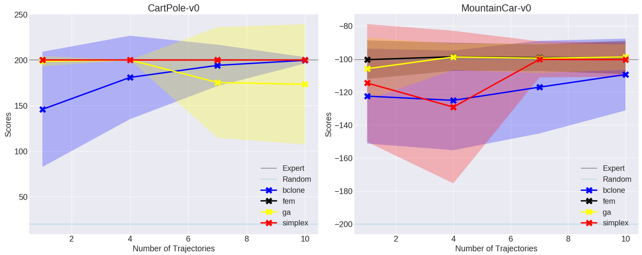
These are comparable with what’s in the paper, though I find it interesting that GAIL seems to choke with the size 7 and 10 datasets for CartPole-v0. Hopefully this is within the random noise. I’ll test with the harder environments shortly.

Acknowledgments: I thank Jonathan Ho for releasing this code. I know it seems like sometimes I (or other users) complain about lack of documentation, but it’s still quite rare to see clean, functional code to exactly reproduce results in research papers. The code base is robust and highly generalizable to various settings. I also learned some new Python concepts from reading his code. Jonathan Ho must be an all-star programmer.

Next Steps: If you’re interested in running the GAIL code sequentially, consider looking at my fork here. I’ve also added considerable documentation.

I have very little experience with programming in clusters, so when OpenAI released their evolution strategies starter code which runs only on EC2 instances, I took this opportunity to finally learn how to program in clusters the way professionals do it.

Amazon Web Services

The first task is to get an Amazon Web Services (AWS) account. AWS offers a mind-bogglingly large amount of resources for doing all sorts of cloud computing. For our purposes, the most important feature is the Elastic Comptue Cloud (EC2). The short description of these guys is that they allow me to run code on heavily-customized machines that I don’t own. The only catch is that running code this way costs some money commensurate with usage, so watch out.

Note that joining AWS means we start off with one year of the free-tier option. This isn’t as good as it sounds, though, since many machines (e.g. those with GPUs) are not eligible for free tier usage. You still have to watch your budget.

One immediate aspect of AWS to understand are their security credentials. They state (emphasis mine):

You use different types of security credentials depending on how you interact with AWS. For example, you use a user name and password to sign in to the AWS Management Console. You use access keys to make programmatic calls to AWS API actions.

To use the OpenAI code, I have to provide my AWS access key and secret access keys, which are officially designated as AWS_ACCESS_KEY_ID and AWS_SECRET_ACCESS_KEY, respectively. These aren’t initialized by default; we have to explicitly create them. This means going to the Security Credentials tab, and seeing:

You can create root access and secret access keys this way, but this is not the recommended way. To be clear, I took the above screenshot during the “root perspective,” so make sure you’re not seeing this on your computer. AWS strongly recommends to instead make a new user with administrative requirements, which effectively means it’s as good as the root account (minus the ability to view billing information). You can see their official instructions here to create groups with administrative privileges. The way I think of it, I’m a systems administrator and have to create a bunch of users for a computer. Except here, I only need to create one. So maybe this is a bit unnecessary, but I think it’s helpful to get used to the good practices as soon as possible. This author even suggests throwing away (!!) the root AWS password.

After following those instructions I had a “new” user and created the two access keys. These must be manually downloaded, where they’ll appear in a .csv file. Don’t lose them!

Next, we have to provide these credentials. When running packer code, as I’ll show in the next section, it suffices to either provide them as command line arguments, or use more secure ways such as adding them to your .bashrc file. I chose the latter. This page from AWS provides further information about how to provide your credentials, and the packer documentation contains similar instructions.

On a final note regarding AWS, I had a hard time figuring out how to actually log in as the Administrator user, rather than the root. This StackOverflow question really helped out, but I’m baffled as to why this isn’t easier to do.

Installing and Understanding Packer

As stated in the OpenAI code, we must use something known as packer to run the code. After installing it, I went through their basic example. Notice that in their .json file, they have the following:

"variables": {
    "aws_access_key": "",
    "aws_secret_key": ""
},

where the access and secret keys must be supplied in some way. They could be hard-coded above if you want to type them in there, but as mentioned earlier, I chose to use environment variables in .bashrc.

Here are a couple of things to keep in mind when running packer’s basic example:

• Be patient when the packer build command is run. It does not officially conclude until one sees:

  ==> Builds finished. The artifacts of successful builds are:
  --> amazon-ebs: AMIs were created:
    
  us-east-1: ami-19601070
  

  where the last line will certainly be different if you run it.

• The output, at least in this case, is an Amazon Machine Image (AMI) that I own. Therefore, I will have to start paying a small fee if this image remains active. There are two steps to deactivating this and ensuring that I don’t have to pay: “deregistering” the image and deleting the (associated) snapshot. For the former, go to the EC2 Management Console and see the IMAGES / AMIs drop-down menu, and for the latter, use ELASTIC BLOCK STORE / Snapshots. From my experience, deregistering can take several minutes, so just be patient. These have to happen in order, as deleting the snapshot first will result in an error which says that the image is still using it.

• When launching (or even when deactivating, for that matter) be careful about the location you’re using. Look at the upper right corner for the locations. The “us-east-1” region is “Northern Virginia” and that is where the image and snapshot will be displayed. If you change locations, you won’t see them.

• Don’t change the “region” argument in the “builders” list; it has to stay at “us-east-1”. When I first fired this up and saw that my image and snapshot were in “us-east-1” instead of the more-desirable “us-west-1” (Northern California) for me, I tried changing that argument and re-building. But then I got an error saying that the image couldn’t be found.

  I think what happens is that the provided “source_ami” argument is the packer author’s fixed, base machine that he set up for the purposes of this tutorial, with packer installed (and maybe some other stuff). Then the .json file we have copies that image, as suggested by this statement in the docs (emphasis mine):

  Congratulations! You’ve just built your first image with Packer. Although the image was pretty useless in this case (nothing was changed about it), this page should’ve given you a general idea of how Packer works, what templates are and how to validate and build templates into machine images.

In packer’s slightly more advanced example, we get to see what happens when we want to pre-install some software on our machines, and it’s here where we see packer’s benefits start to truly shine. In that new example, the “provisions” list lets us run command line arguments to install desired packages (i.e. sudo apt-get install blahblahblah). When I ssh-ed into the generated machine — a bit of a struggle at first since I didn’t realize the username to get in was actually ubuntu instead of ec2-user — I could successfully run redis-server on the command line and it was clear that the package had been installed.

In OpenAI’s code, they have a full script of commands which they load in. Thus, any image that we create from the packer build will have those commands run, so that our machines will have exactly the kind of software we want. In particular, OpenAI’s script installs TensorFlow, gym, the ALE, and so on. If we didn’t have packer, I think we would have to manually execute that script for all the machines. To give a sense of how slow that would be, the OpenAI ES paper said they once tested with 1,440 machines.

OpenAI’s Code

The final stage is to understand how to run OpenAI’s code. As mentioned earlier, there’s a dependency.sh shell script which will install stuff on our cloud-computing machines. Unfortunately, MuJoCo is not open source. (Fortunately, we might have an alternative with OpenAI’s RoboSchool — I hope to see that work out!) Thus, we have to add our own license. For me, this was a two-stage process.

First, in the configuration file, I added the following two file provisioners:

"provisioners": [
  {   
    "type": "file",
    "source": "/home/daniel/mjpro131",
    "destination": "~/"
  },  
  {   
    "type": "file",
    "source": "/home/daniel/mjpro131/mjkey.txt",
    "destination": "~/"
  },  
  {   
    "type": "shell",
    "scripts": [
      "dependency.sh"
    ]
  }   
]

In packer, the elements in the “provisioners” array are executed in order of their appearance, so I wanted the files sent over to the home directory on the images so that they’d be there for the shell script later. The “source” strings are where MuJoCo is stored on my personal machine, the one which executes packer build packer.json.

Next, inside dependency.sh, I simply added the following two sudo mv commands:

#######################################################
# WRITE CODE HERE TO PLACE MUJOCO 1.31 in /opt/mujoco #
# The key file should be in /opt/mujoco/mjkey.txt     #
# Mujoco should be installed in /opt/mujoco/mjpro131  #
#######################################################
sudo mv ~/mjkey.txt /opt/mujoco/
sudo mv ~/mjpro131 /opt/mujoco/

(Yes, we’re still using MuJoCo 1.31. I’m not sure why the upgraded versions don’t work.)

This way, when running packer build packer.json, the relevant portion of the output should look something like this:

amazon-ebs: + sudo mkdir -p /opt/mujoco
amazon-ebs: + sudo mv /home/ubuntu/mjkey.txt /opt/mujoco/
amazon-ebs: + sudo mv /home/ubuntu/mjpro131 /opt/mujoco/
amazon-ebs: + sudo tee /etc/profile.d/mujoco.sh
amazon-ebs: + sudo echo 'export MUJOCO_PY_MJKEY_PATH=/opt/mujoco/mjkey.txt'
amazon-ebs: + sudo tee -a /etc/profile.d/mujoco.sh
amazon-ebs: + sudo echo 'export MUJOCO_PY_MJPRO_PATH=/opt/mujoco/mjpro131'
amazon-ebs: + . /etc/profile.d/mujoco.sh

where the sudo mv commands have successfully moved my MuJoCo materials over to the desired target directory.

As an aside, I should also mention the other change I made to packer.json: in the “ami_regions” argument, I deleted all regions except for “us-west-1”, since otherwise images would be created in all the regions listed.

Running packer build packer.json takes about thirty minutes to run. Upon concluding, I saw the following output:

==> Builds finished. The artifacts of successful builds are:
--> amazon-ebs: AMIs were created:

us-west-1: ami-XXXXXXXX

where for security reasons, I have not revealed the full ID. Then, inside launch.py, I put in:

# This will show up under "My AMIs" in the EC2 console.
AMI_MAP = {
    "us-west-1": "ami-XXXXXXXX"
} 

The last step is to call the launcher script with the appropriate arguments. Before doing so, make sure you’re using Python 3. I originally ran this with Python 2.7 and was getting some errors. (Yeah, yeah, I still haven’t changed even though I said I would do so four years ago; blame backwards incompatibility.) One easy way to manage different Python versions on one machine is to use Python virtual environments. I started a new one with Python 3.5 and was able to get going after a few pip install commands.

You can find the necessary arguments in the main method of launch.py. To understand these arguments, it can be helpful to look at the boto3 documentation, which is the Python library that interfaces with AWS. In particular, reading the create_instances documentation will be useful.

I ended up using:

python launch.py ../configurations/humanoid.json \
    --key_name="MyKeyPair" \
    --s3_bucket="s3://put-name-here" \
    --region_name="us-west-1" \
    --zone="us-west-1b" \
    --master_instance_type="m4.large" \
    --worker_instance_type="t2.micro" \
    --security_group="default" \
    --spot_price="0.05"

A few pointers:

• Make sure you run sudo apt install awscli if you don’t have the package already installed.
• Double check the default arguments for the two access keys. They’re slightly different than what I used in the packer example, so I adjusted my .bashrc file.
• “MyKeyPair” comes from the MyKeyPair.pem file which I created via the EC2 console.
• The s3_bucket argument is based on AWS Simple Storage Service. I made my own unique bucket name via the S3 console, and to actually provide it as an argument, write it as s3://put-name-here where put-name-here is what you created.
• The region_name should be straightforward. The zone argument is similar, except we add letters at the end since they can be thought of as “subsets” of the regions. Not all zones will be available to you, since AWS adjusts what you can use so that it can more effectively achieve load balancing for its entire service.
• The master_instance_type and worker_instance_type arguments are the names of the instance types; see this for more information. It turns out that the master requires a more advanced (and thus more expensive) type due to EBS optimization. I chose t2.micro for the workers, which seems to work and is better for me since that’s the only type eligible for the free tier.
• The security_groups you have can be found in the EC2 console under NETWORK & SECURITY / Security Groups. Make sure you use the name, not the ID; the names are NOT the strings that look like “sg-XYZXYZXYZ”. Watch out!

• Finally, the spot_price indicates the maximum amount to bid, since we’re using “Spot Instances” rather than “On Demand” pricing. OpenAI’s README says:

  It’s resilient to worker termination, so it’s safe to run the workers on spot instances.

  The README says that because spot instances can be terminated if we are out-bid.

By the way, to be clear on what I mean when I talk about the “EC2 Console” and “S3 Console”, here’s the general AWS console:

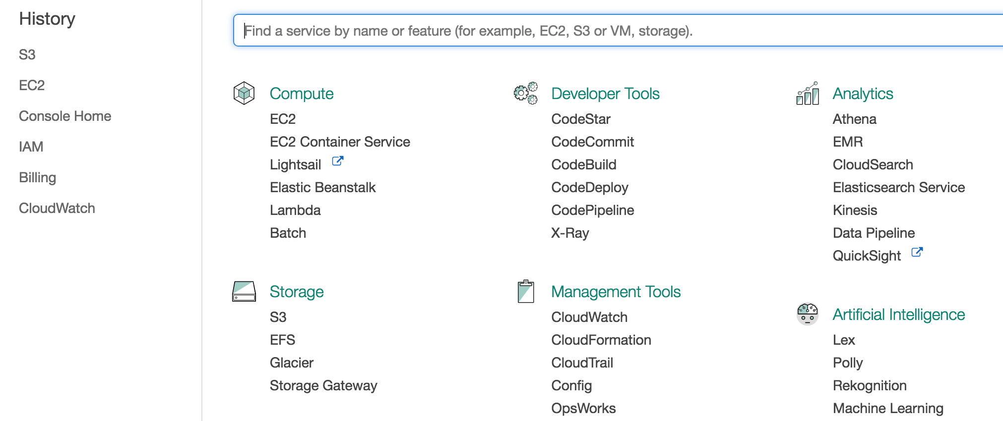
The desired consoles can be accessed by clicking “EC2” or “S3” in the above.

If all goes well, you should see a message like this:

Scaling group created
humanoid_20170530-133848 launched successfully.
Manage at [Link Removed]

Copy and paste the link in your browser, and you will see your instance there, running OpenAI’s code.

Back in Fall 2015, I took the first edition of Deep Reinforcement Learning (CS 294-112) at Berkeley. As usual, I wrote a blog post about the class; you can find more about other classes I’ve taken by searching the archives.

In that blog post, I admitted that CS 294-112 had several weaknesses, and also that I didn’t quite fully understand the material. Fast forward to today, and I’m pleased to say that:

• There has been a second edition of CS 294-112, taught this past spring semester. It was a three-credit, full semester course and therefore more substantive than the previous edition which was two-credits and lasted only eight weeks. Furthermore, the slides, homework assignments, and the lecture recordings are all publicly available online. Check out the course website for details. You can find the homework assignments in this GitHub repository (I had to search a bit for this).

• I now understand much more about deep reinforcement learning and about how to use TensorFlow.

These developments go hand in hand, because I spent much of the second half of the Spring 2017 semester self-studying the second edition of CS 294-112. (To be clear, I was not enrolled in the class.) I know I said I would first self-study a few other courses in a previous blog post, but I couldn’t pass up such a prime opportunity to learn about deep reinforcement learning. Furthermore, the field moves so fast that I worried that if I didn’t follow what was happening now, I would never be able to catch up to the research frontier if I tried to do so in a year.

The class had four homework assignments, and I completed all of them with the exception of skipping the DAgger algorithm implementation in the first homework. The assignments were extremely helpful for me to understand how to better use TensorFlow, and I finally feel comfortable using it for my personal projects. If I can spare the time (famous last words) I plan to write some TensorFlow-related blog posts.

The video lecture were a nice bonus. I only watched a fraction of them, though. This was in part due to time constraints, but also in part due to the lack of captions. The lecture recordings are on YouTube, and in YouTube, I can turn on automatic captions which helps me to follow the material. However, some of the videos didn’t enable that option, so I had to skip those and just read the slides since I wasn’t following what was being said. As far as I remember, automatic captions are provided as an option so long as whoever uploaded the video enables some setting, so maybe someone forgot to do so? Fortunately, the lecture video on policy gradients has captions enabled, so I was able to watch that one. Oh, and I wrote a blog post about the material.

Another possible downside to the course, though this one is extremely minor, is that the last few class sessions were not recorded, since those were when students presented their final projects. Maybe the students wanted some level of privacy? Oh well, I suppose there’s way too many other interesting projects available anyway (by searching GitHubs, arXiv preprints, etc.) to worry about this thing.

I want to conclude with a huge thank you to the course staff. Thank you for helping to spread knowledge about deep reinforcement learning with a great class and with lots of publicly available material. I really appreciate it.

I finished reading Andrew Hodges’ book Alan Turing: The Engima, otherwise known as the definitive biography of mathematician, computer scientist, and code breaker Alan Turing. I was inspired to read the book in part because I’ve been reading lots of AI-related books this year¹ and in just about every one of those books, Alan Turing is mention in some form. In addition, I saw the film The Imitation Game, and indeed this is the book that inspired it. I bought the 2014 edition of the book — with The Imitation Game cover — during a recent visit to the National Cryptology Museum.

The author is Andrew Hodges, who at that time was a mathematics instructor at the University of Oxford (he’s now retired). He maintains a website where he commemorates Alan Turing’s life and achievements. I encourage the interested reader to check it out. Hodges has the qualifications to write about the book, being deeply versed in mathematics. He also appears to be gay himself.²

After reading the book, my immediate thoughts relating to the positive aspects of the books are:

• The book is organized chronologically and the eight chapters are indicated with date ranges. Thus, for a biography of this size, it is relatively straightforward to piece together a mental timeline of Alan Turing’s life.

• The book is detailed. Like, wow. The edition I have is 680 pages, not counting the endnotes at the back of the book which command an extra 30 or so pages. Since I read almost every word of this book (I skipped a few endnotes), and because I tried to stay alert when reading this book, I felt like I got a clear picture of Turing’s life, along with what life must have been like during the World War II-era.

• The book contains quotes and writings from Turing that show just how far ahead of his time he was. For instance, even today people are still utilizing concepts from his famous 1936 paper On Computable Numbers, with an Application to the Entscheidungsproblem and his 1950 paper Computing Machinery and Intelligence. The former introduced Turing Machines, the latter introduced the famous Turing Test. Fortunately, I don’t think there was much exaggeration of Turing’s accomplishments, unlike the The Imitation Game. When I was reading his quotes, I often had to remind myself that “this is the 1940s or 1950s ….”

• The book showcases the struggles of being gay, particularly during a time when homosexual activity was a crime. The book actually doesn’t seem to cover some of his struggles in the early 1950s as much as I thought it would be, but it was probably difficult to find sufficient references for this aspect of his life. At the very least, readers today should appreciate how much our attitude towards homosexuality has improved.

That’s not to say there weren’t a few downsides. Here are some I thought of:

• Related to what I mentioned earlier, it is long. It too me a month to finish, and the writing is in “1983-style” which makes it more difficult for me to understand. (By contrast, I read both of Richard Dawkins’ recent autobiographies, which combine to be roughly the same length as Hodges’ book, and Dawkins’ books were much easier to read.) Now, I find Turing’s life very interesting so this is more of a “neutral” factor to me, but I can see why the casual reader might be dissuaded from reading this book.

• Much of the material is technical even to me. I understand the basics of Turing Machines but certainly not how the early computers were built. The hardest parts of the book to read are probably in chapters six and seven (out of eight total). I kept asking to myself “what’s a cathode ray”?

To conclude, the book is an extremely detailed overview of Turing’s life which at times may be technically challenging to read.

I wonder what Alan Turing would think about AI today. The widely-used AI undergraduate textbook by Stuart Russell and Peter Norvig concludes with the follow prescient quote by Turing:

We can only see a short distance ahead, but we can see plenty there that needs to be done.

Earlier scientists have an advantage in setting their legacy in their fields since it’s easier to make landmark contributions. I view Charles Darwin, for instance, as the greatest biologist who has ever lived, and no matter how skilled today’s biologists are, I believe none will ever be able to surpass Darwin’s impact. The same goes today for Alan Turing, who (possibly along with John von Neumann) is one of the two preeminent computer scientists who has ever lived.

Despite all the talent that’s out there in computer science, I don’t think any one individual can possibly surpass Turing’s legacy on computer science and artificial intelligence.

The paper “Understanding Deep Learning Requires Rethinking Generalization” (arXiv link) caused quite a stir in the Deep Learning and Machine Learning research communities. It’s the rare paper that seems to have high research merit — judging from being awarded one of three Best Paper awards at ICLR 2017 — but is also readable. Hence, it got the most amount of comments of any ICLR 2017 submission on OpenReview. It has also been discussed on reddit and was recently featured on The Morning Paper blog. I was aware of the paper shortly after it was uploaded to arXiv, but never found the time to read it in detail until now.

I enjoyed reading the paper, and while I agree with many readers that some of the findings might be obvious, the paper nonetheless seems deserving of the attention it has been getting.

The authors conveniently put two of their important findings in centered italics:

Deep neural networks easily fit random labels.

and

Explicit regularization may improve generalization performance, but is neither necessary nor by itself sufficient for controlling generalization error.

I will also quote another contribution from the paper that I find interesting:

We complement our empirical observations with a theoretical construction showing that generically large neural networks can express any labeling of the training data.

(I go through the derivation later in this post.)

Going back to their first claim about deep neural networks fitting random labels, what does this mean from a generalization perspective? (Generalization is just the difference between training error and testing error.) It means that we cannot come up with a “generalization function” that can take in a neural network as input and output a generalization quality score. Here’s my intuition:

• What we want: let’s imagine an arbitrary encoding of a neural network designed to give as much deterministic information as possible, such as the architecture and hyperparameters, and then use that encoding as input to a generalization function. We want that function to give us a number representing generalization quality, assuming that the datasets are allowed to vary. The worst generalization occurs when a fixed neural network gets excellent training error but could get either the same testing error (awesome!), or get test-set performance no better than random guessing (ugh!).

• Reality: unfortunately, the best we can do seems to be no better than the worst case. We know of no function that can provide bounds on generalization performance across all datasets. Why? Let’s use the LeNet architecture and MNIST as an example. With the right architecture, generalization error is very small as both training and testing performance are in the high 90 percentages. With a second data set that consists of the same MNIST digits, but with the labels randomized, that same LeNet architecture can do no better than random guessing on the test set, even though the training performance is extremely good (or at least, it should be). That’s literally as bad as we can get. There’s no point in developing a function to measure generalization when we know it can only tell us that generalization will be in between zero (i.e. perfect) and the difference between zero and random guessing (i.e. the worst case)!

As they later discuss in the paper, regularization can be used to improve generalization, but will not be sufficient for developing our desired generalization criteria.

Let’s briefly take a step back and consider classical machine learning, which provides us with generalization criteria such as VC-dimension, Rademacher complexity, and uniform stability. I learned about VC-dimension during my undergraduate machine learning class, Rademacher complexity during STAT 210B this past semester, and … actually I’m not familiar with uniform stability. But intuitively … it makes sense to me that classical criteria do not apply to deep networks. To take the Rademacher complexity example: a function class which can fit to arbitrary \(\pm 1\) noise vectors presents the trivial bound of one, which is like saying: “generalization is between zero and the worst case.” Not very helpful.

The paper then proceeds to describe their testing scenario, and packs some important results in the figure reproduced below:

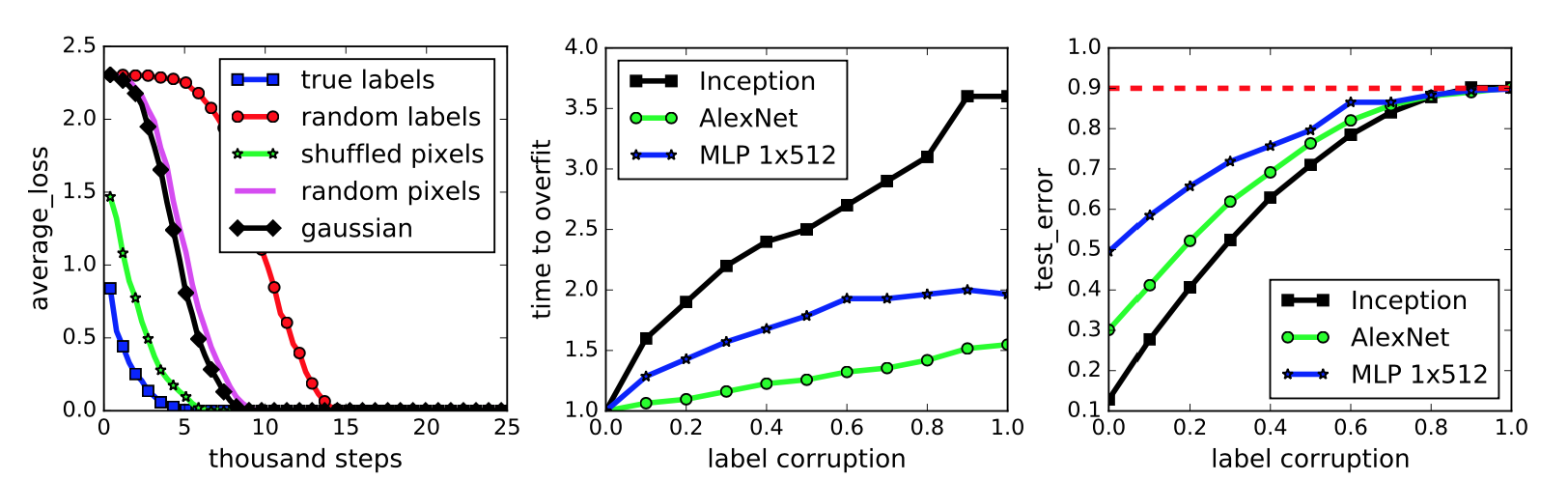
This figure represents a neural network classifying the images in the widely-benchmarked CIFAR-10 dataset. The network the authors used is a simplified version of the Inception architecture.

• The first subplot represents five different settings of the labels and input images. To be clear on what the “gaussian” setting means, they use a Gaussian distribution to generate random pixels (!!) for every image. The mean and variance of that Gaussian are “matched to the original dataset.” In addition, the “shuffled” and “random” pixels apply a random permutation to the pixels, with the same permutation to all images for the former, and different permutations for the latter.

  We immediately see that the neural network can get zero training error on all the settings, but the convergence speed varies. Intuition suggests that the dataset with the correct labels and the one with the same shuffling permutation should converge quickly, and this indeed is the case. Interestingly enough, I thought the “gaussian” setting would have the worst performance, but that prize seems to go to “random labels.”

• The second subplot measures training error when the amount of label noise is varied; with some probability \(p\), each image independently has its labeled corrupted and replaced with a draw from the discrete uniform distribution over the classes. The results show that more corruption slows convergence, which makes sense. By the way, using a continuum of something is a common research tactic and something I should try for my own work.

• Finally, the third subplot measures generalization error under label corruption. As these data points were all measured after convergence, this is equivalent to the test error. The results here also make a lot of sense. Test set error should be approaching 90 percent because CIFAR-10 has 10 classes (that’s why it’s called CIFAR-10!).

My major criticism of this figure is not that the results, particularly in the second and third subplots, might seem obvious but that the figure lacks error bars. Since it’s easy nowadays to program multiple calls in a bash script or something similar, I would expect at least three trials and with error bars (or “regions”) to each curve in this figure.

The next section discusses the role of regularization, which is normally applied to prevent overfitting to the training data. The classic example is with linear regression and a dataset of several points arranged in roughly a linear fashion. Do we try to fit a straight line through these points, which might have lots of training error, or do we take a high-dimensional polynomial and fit every point exactly, even if the resulting curve looks impossibly crazy? That’s what regularization helps to control. Explicit regularization in linear regression is the \(\lambda\) term in the following optimization problem:

I presented this in an earlier blog post.

To investigate the role of regularization in Deep Learning, the authors test with and without regularizers. Incidentally, the use of \(\lambda\) above is not the only type of regularization. There are also several others: data augmentation, dropout, weight decay, early stopping (implicit) and batch normalization (implicit). These are standard tools in the modern Deep Learning toolkit.

They find that, while regularization helps to improve generalization performance, it is still possible to get excellent generalization even with no regularization. They conclude:

In summary, our observations on both explicit and implicit regularizers are consistently suggesting that regularizers, when properly tuned, could help to improve the generalization performance. However, it is unlikely that the regularizers are the fundamental reason for generalization, as the networks continue to perform well after all the regularizers [are] removed.

On a side note, the regularization discussion in the paper feels out of order and the writing sounds a bit off to me. I wish they had more time to fix this, as the regularization portion of the paper contains most of my English language-related criticism.

Moving on, the next section of the paper is about finite-sample expressivity, or understanding what functions neural networks can express given a finite number of samples. The authors state that the previous literature focuses on population analysis where one can assume an arbitrary number of samples. Here, instead, they assume a fixed set of \(n\) training points \(\{x_1,\ldots,x_n\}\). This seems easier to understand anyway.

They prove a theorem that relates to the third major contribution I wrote earlier: “that generically large neural networks can express any labeling of the training data.” Before proving the theorem, let’s begin with the following lemma:

Lemma 1. For any two interleaving sequences of \(n\) real numbers

\[b_1 < x_1 < b_2 < x_2 \cdots < b_n < x_n\]

the \(n \times n\) matrix \(A = [\max\{x_i - b_j, 0\}]_{ij}\) has full rank. Its smallest eigenvalue is \(\min_i (x_i - b_i)\).

Whenever I see statements like these, my first instinct is to draw out the matrix. And here it is:

where (i) follows from the interleaving sequence assumption. This matrix is lower-triangular, and moreover, all the non-zero elements are positive. We know from linear algebra that lower triangular matrices

• are invertible if and only if the diagonal elements are nonzero
• have their eigenvalues taken directly from the diagonal elements

These two facts together prove Lemma 1. Next, we can prove:

Theorem 1. There exists a two-layer neural network with ReLU activations and \(2n + d\) weights that can represent any function on a sample of size \(n\) in \(d\) dimensions.

Consider the function

with \(w, b \in \mathbb{R}^n\) and \(a,x\in \mathbb{R}^d\). (There’s a typo in the paper, \(c\) is a function from \(\mathbb{R}^d\to \mathbb{R}\), not \(\mathbb{R}^n\to \mathbb{R}\)). This can certainly be represented by a depth-2 ReLU network. To be clear on the naming convention, “depth-2” does not count the input layer, so our network should only have one ReLU layer in it as the output shouldn’t have ReLUs applied to it.

Here’s how to think of the network representing \(c\). First, assume that we have a minibatch of \(n\) elements, so that \(X\) is the \(n\times d\) data matrix. The depth-2 network representing \(c\) can be expressed as:

where \(b\) and the zero-vector used in the maximum “broadcast” as necessary in Python code.

Given a fixed dataset \(S=\{z_1,\ldots,z_n\}\) of distinct inputs with labels \(y_1,\ldots,y_n\), we must be able to find settings of \(a,w,\) and \(b\) such that \(c(z_i)=y_i\) for all \(i\). You might be guessing how we’re doing this: we must reduce this to the interleaving property in Lemma 1. Due to the uniqueness of the \(z_i\), it is possible to find \(a\) to make the \(x_i=z_i^Ta\) terms satisfy the interleaving property. Then we have a full rank solution, hence \(y=Aw\) results in \(w^* = A^{-1}y\) as our final weights, where \(A\) is precisely that matrix from Lemma 1! We also see that, indeed, there are \(n+n+d\) weights in the network. This is an interesting and fun proof, and I think variants of this question would work well as a homework assignment for a Deep Learning class.

The authors conclude the paper by trying to understand generalization with linear models, in the hope that some of the intuition will transfer over to the Deep Learning setting. With linear models, given some weights \(w\) resulting from the optimization problem, what can we say about generalization just by looking at it? Curvature is one popular metric to understand the quality of the minima (which is not necessarily the same as the generalization criteria!), but the Hessian is independent of \(w\), so in fact it seems impossible to use curvature for generalization. I’m convinced this is true for the normal mean square loss, but is this still true if the loss function were, say, the cube of the \(L_2\) difference? After all, there are only two derivatives applied on \(w\), right?

The authors instead urge us to think of stochastic gradient descent instead of curvature when trying to measure quality. Assuming that \(w_0=0\), the stochastic gradient descent update consists of a series of “linear combination” updates, and hence the result is just a linear combination of linear combinations of linear combinations … (and so forth) … which at the end of the day, remains a linear combination. (I don’t think they need to assume \(w_0=0\) if we can add an extra 1 to all the data points.) Consequently, they can fit any set of labels of the data by solving a linear equation, and indeed, they get strong performance on MNIST and CIFAR-10, even without regularization.

They next try to relate this to a minimum norm interpretation, though this is not a fruitful direction because their results are worse when they try to find minimum norm solutions. On MNIST, their best solution using some “Gabor wavelet transform” (what?), is twice as better as the minimum norm solution. I’m not sure how much stock to put into this section, other than how I like their perspective of thinking of SGD as an implicit regularizer (like batch normalization) rather than an optimizer. The line between the categories is blurring.

To conclude, from my growing experience with Deep Learning, I don’t find their experimental results surprising. That’s not to say the paper was entirely predictable, but think of it this way: if I were a computer vision researcher pre-AlexNet, I would be more surprised at reading the AlexNet paper as I am today reading this paper. Ultimately, as I mentioned earlier, I enjoyed this paper, and while it was predictable (that word again…) that it couldn’t offer any solutions, perhaps it will be useful as a starting point to understanding generalization in Deep Learning.

I have passionately studied various machine learning and statistical concepts over the last few years. One thing I’ve learned from all this is that there are many mathematical “tricks” involved, whether or not they are explicitly stated. (In research papers, such tricks are often used without acknowledgment since it is assumed that anyone who can benefit from reading the paper has the mathematical maturity to fill in the details.) I thought it would be useful for me, and hopefully for a few interested readers, to catalogue a set of the common tricks here, and to see them applied in a few examples.

The following list, in alphabetical order, is a non-exhaustive set of tricks that I’ve seen:

• Cauchy-Schwarz
• Integrating Probabilities into Expectations
• Introducing an Independent Copy
• Jensen’s Inequality
• Law of Iterated Expectation
• Lipschitz Functions
• Markov’s Inequality
• Norm Properties
• Series Expansions (e.g. Taylor’s)
• Stirling’s Approximation
• Symmetrization
• Take a Derivative
• Union Bound
• Variational Representations

If the names are unclear or vague, the examples below should clarify. All the tricks are used except for the law of iterated expectation, i.e. \(\mathbb{E}[\mathbb{E}[X|Y]] = \mathbb{E}[X]\). (No particular reason for that omission; it just turns out the exercises I’m interested in didn’t require it.)

Example 1: Maximum of (Not Necessarily Independent!) sub-Gaussians

I covered this problem in my last post here so I will not repeat the details. However, there are two extensions to that exercise which I thought would be worth noting.

First, To prove an upper bound for the random variable \(Z = \max_{i=1,2,\ldots,n}|X_i|\), it suffices to proceed as we did earlier in the non-absolute value case, but augment our sub-Gaussian variables \(X_1,\ldots,X_n\) with the set \(-X_1,\ldots,-X_n\). It’s OK to do this because no independence assumptions are needed. Then it turns out that an upper bound can be derived as

This is the same as what we had earlier, except the “2” is now outside the square root. It’s quite intuitive.

Second, consider how we can prove the following bound:

We start by applying the standard technique of multiplying by \(\lambda>0\), exponentiating and then applying Markov’s Inequality with our non-negative random variable \(e^{\lambda Z}\):

where in (i) we used a bound previously determined in our bound on \(\mathbb{E}[Z]\) (it came out of an intermediate step), and then used the fact that the term in the exponential is a convex quadratic to find the minimizer value \(\lambda^* = \frac{\delta+2\sqrt{\sigma^2 \log n}}{\sigma^2}\) via differentiation in (ii).

At this point, to satisfy the desired inequality, we compare terms in the exponentials and claim that with \(\delta \ge 0\),

This will result in our desired bound. It therefore remains to prove this, but it reduces to checking that

and the left hand side is non-negative. Hence, the desired bound holds.

Tricks used:

• Jensen’s Inequality
• Markov’s Inequality
• Take a Derivative
• Union Bound

Comments: My earlier blog post (along with this one) shows what I mean when I say “take a derivative.” It happens when there is an upper bound on the right hand side and we have a free parameter \(\lambda \in \mathbb{R}\) (or \(\lambda \ge 0\)) which we can optimize to get the tighest possible bound. Often times, such a \(\lambda\) is explicitly introduced via Markov’s Inequality, as we have here. Just make sure to double check that when taking a derivative, you’re getting a minimum, not a maximum. In addition, Markov’s Inequality can only be applied to non-negative random variables, which is why we often have to exponentiate the terms inside a probability statement first.

Note the use of convexity of the exponential function. It is very common to see Jensen’s inequality applied with the exponential function. Always remember that \(e^{\mathbb{E}[X]} \le \mathbb{E}[e^X]\)!!

The procedure that I refer to as the “union bound” when I bound a maximum by a sum isn’t exactly the canonical way of doing it, since that typically involves probabilities, but it has a similar flavor. More formally, the union bound states that

for countable sets of events \(A_1,A_2,\ldots\). When we define a set of events based on a maximum of certain variables, that’s the same as taking the union of the individual events.

On a final note, be on the look-out for applications of this type whenever a “maximum” operation is seen with something that resembles Gaussians. Sometimes this can be a bit subtle. For instance, it’s not uncommon to use a bound of the form above when dealing with \(\mathbb{E}[\|w\|_\infty]\), the expectation of the \(L_\infty\)-norm of a standard Gaussian vector. In addition, when dealing with sparsity, often our “\(n\)” or “\(d\)” is actually something like \({d \choose s}\) or another combinatorics-style value. Seeing a “log” accompanied by a square root is a good clue and may help identify such cases.

Example 2: Bounded Random Variables are Sub-Gaussian

This example is really split into two parts. The first is as follows:

Prove that Rademacher random variables are sub-Gaussian with parameter \(\sigma = 1\).

The next is:

Prove that if \(X\) is a zero-mean and has support \(X \in [a,b]\), then \(X\) is sub-Gaussian with parameter (at most) \(\sigma = b-a\).

To prove the first part, let \(\varepsilon\) be a Rademacher random variable. For \(\lambda \in \mathbb{R}\), we have

and thus the claim is satisfied by the definition of a sub-Gaussian random variable. In (i), we removed the expectation by using facts from Rademacher random variables, in (ii) we used the series expansions of the exponential function, in (iii) we simplified by removing the odd powers, in (iv) we used the clever trick that \(2^kk! \le (2k)!\), and in (v) we again used the exponential function’s power series.

To prove the next part, observe that for any \(\lambda \in \mathbb{R}\), we have

which shows by definition that \(X\) is sub-Gaussian with parameter \(\sigma = b-a\). In (i), we cleverly introduce an extra independent copy \(X'\) inside the exponent. It’s zero-mean, so we can insert it there without issues.¹ In (ii), we use Jensen’s inequality, and note that we can do this with respect to just the random variable \(X'\). (If this is confusing, just think of the expression as a function of \(X'\) and ignore the outer expectation.) In (iii) we apply a clever symmetrization trick by multiplying a Rademacher random variable to \(X-X'\). The reason why we can do this is that \(X-X'\) is already symmetric about zero. Hence, inserting the Rademacher factor will maintain that symmetry (since Rademachers are only +1 or -1). In (iv), we applied the Rademacher sub-Gaussian bound with \(X-X'\) held fixed, and then in (v), we finally use the fact that \(X,X' \in [a,b]\).

Tricks used:

• Introducing an Independent Copy
• Jensen’s Inequality
• Series Expansions (twice!!)
• Symmetrization

Comments: The first part is a classic exercise in theoretical statistics, one which tests your ability to understand how to use the power series of exponential functions. The first part involved converting an exponential function to a power series, and then later doing the reverse. When I was doing this problem, I found it easiest to start by stating the conclusion — that we would have \(e^{\frac{\lambda^2}{2}}\) somehow — and then I worked backwards. Obviously, this only works when the problem gives us the solution!

The next part is also “classic” in the sense that it’s often how students (such as myself) are introduced to the symmetrization trick. The takeaway is that one should be on the lookout for anything that seems symmetric. Or, failing that, perhaps introduce symmetry by adding in an extra independent copy, as we did above. But make sure that your random variables are zero-mean!!

Example 3: Concentration Around Median and Means

Here’s the question:

Given a scalar random variable \(X\), suppose that there are positive constants \(c_1,c_2\) such that

\[\mathbb{P}[|X-\mathbb{E}[X]| \ge t] \le c_1e^{-c_2t^2}\]

for all \(t \ge 0\).

(a) Prove that \({\rm Var}(X) \le \frac{c_1}{c_2}\)

(b) Prove that for any median \(m_X\), we have

\[\mathbb{P}[|X-m_X| \ge t] \le c_3e^{-c_4t^2}\]

for all \(t \ge 0\), where \(c_3 = 4c_1\) and \(c_4 = \frac{c_2}{8}\).

To prove the first part, note that

where (i) follows from definition, (ii) follows from the “integrating probabilities into expectations” trick (which I will describe shortly), (iii) follows from the provided bound, and (iv) follows from standard calculus (note the multiplication of \(c_2/c_2\) for mathematical convenience). This proves the first claim.

This second part requires some clever insights to get this to work. One way to start is by noting that:

and where the last inequality follows from the bound provided in the question. For us to be able to apply that bound, assume without loss of generality that \(m_X \ge \mathbb{E}[X]\), meaning that our \(t = m_X-\mathbb{E}[X]\) term is positive and that we can increase the probability by inserting in absolute values. The above also shows that

We next tackle the core of the question. Starting from the left hand side of the desired bound, we get

where step (i) follows from adding zero, step (ii) follows from the Triangle Inequality, and (iii) follows from the provided bound based on the expectation. And yes, this is supposed to work only for when \(t-|\mathbb{E}[X]-m_X| > 0\). The way to get around this is that we need to assume \(t\) is greater than some quantity. After some algebra, it turns out a nice condition for us to enforce is that \(t > \sqrt{\frac{8\log(4c_1)}{c_2}}\), which in turn will make \(t-|\mathbb{E}[X]-m_X| > 0\). If \(t < \sqrt{\frac{8\log(4c_1)}{c_2}}\), then the desired bound is attained because

a fact which can be derived through some algebra. Thus, the remainder of the proof boils down to checking the case that when \(t > \sqrt{\frac{8\log(4c_1)}{c_2}}\), we have

and this is proved by analyzing roots of the quadratic and solving for \(t\).

Tricks used:

• Integrating Probabilities into Expectations
• Triangle Inequality

Comments: The trick “integrating probabilities into expectations” is one which I only recently learned about, though one can easily find it (along with the derivation) on the Wikipedia page for the expected values. In particular, note that for a positive real number \(\alpha\), we have

and in the above, I use this trick with \(\alpha=2\). It’s quite useful to convert between probabilities and expectations!

The other trick above is using the triangle inequality in a clever way. The key is to observe that when we have something like \(\mathbb{P}[X\ge Y]\), if we increase the value of \(X\), then we increase that probability. This is another common trick used in proving various bounds.

Finally, the above also shows that when we have constants \(t\), it pays to be clever in how we assign those values. Then the remainder is some brute-force computation. I suppose it also helps to think about inserting \(1/2\)s whenever we have a probability and a median.

Example 4: Upper Bounds for \(\ell_0\) “Balls”

Consider the set

We often write the number of nonzeros in \(\theta\) as \(\|\theta\|_0\) like this even though \(\|\cdot\|_0\) is not technically a norm. This exercise consists of three parts:

(a) Show that \(\mathcal{G}(T^d(s)) = \mathbb{E}[\max_{\mathcal{S}} \|w_S\|_2]\) where \(\mathcal{S}\) consists of all subsets \(S\) of \(\{1,2,\ldots, d\}\) of size \(s\), and \(w_S\) is a sub-vector of \(w\) (of size \(s\)) indexed by those components. Note that by this definition, the cardinality of \(\mathcal{S}\) is equal to \({d \choose s}\).

(b) Show that for any fixed subset \(S\) of cardinality \(s\), we have \(\mathbb{P}[\|w_S\|_2 \ge \sqrt{s} + \delta] \le e^{-\frac{\delta^2}{2}}\).

(c) Establish the claim that \(\mathcal{G}(T^d(s)) \precsim \sqrt{s \log \left(\frac{ed}{s}\right)}\).

To be clear on the notation, \(\mathcal{G}(T^d(s)) = \mathbb{E}\left[\sup_{\theta \in T^d(s)} \langle \theta, w \rangle\right]\) and refers to the Gaussian complexity of that set. It is, roughly speaking, a way to measure the “size” of a set.

To prove (a), let \(\theta \in T^d(s)\) and let \(S\) indicate the support of \(\theta\) (i.e. where its nonzeros occur). For any \(w \in \mathbb{R}^d\) (which we later treat to be sampled from \(N(0,I_d)\), though the immediate analysis below does not require that fact) we have

where \(\tilde{\theta}\in \mathbb{R}^s\) refers to the vector taking only the nonzero components from \(\theta\). The first inequality follows from Cauchy-Schwarz. In addition, by standard norm properties, taking \(\theta = \frac{w_S}{\|w_S\|_2} \in T^d(s)\) results in the case when equality is attained. The claim thus follows. (There are some technical details needed regarding which of the maximums — over the set sizes or over the vector selection — should come first, but I don’t think the details are critical for me to know.)

For (b), we first claim that the function \(f_S : \mathbb{R}^d \to \mathbb{R}\) defined as \(f_S(w) := \|w_S\|_2\) is Lipschitz with respect to the Euclidean norm with Lipschitz constant \(L=1\). To see this, observe that when \(w\) and \(w'\) are both \(d\)-dimensional vectors, we have

where (i) follows from the reverse triangle inequality for normed spaces and (ii) follows from how the vector \(w_S-w_S'\) cannot have more nonzero terms than \(w-w'\) but must otherwise match it for indices lying in the subset \(S\).

The fact that \(f_S\) is Lipschitz means that we can apply a theorem regarding tail bounds of Lipschitz functions of Gaussian variables. The function \(f_S\) here doesn’t require its input to consist of vectors with IID standard Gaussian components, but we have to assume that the input is like that for the purposes of the theorem/bound to follow. More formally, for all \(\delta \ge 0\) we have

where (i) follows from how \(\mathbb{E}[\|w_S\|_2] \le \sqrt{s}\) and thus we are just decreasing the threshold for the event (hence making it more likely) and (ii) follows from the theorem, which provides an \(L\) in the denominator of the exponential, but \(L=1\) here.

Finally, to prove (c), we first note that the previous part’s theorem guaranteed that the function \(f_S(w) = \|w_S\|_2\) is sub-Gaussian with parameter \(\sigma=L=1\). Using this, we have

where (i) applies the bound for a maximum over sub-Gaussian random variables \(\|w_S\|_2\) for all the \({d\choose s}\) sets \(S \in \mathcal{S}\) (see Example 1 earlier), each with parameter \(\sigma\), and (ii) applies an approximate bound due to Stirling’s approximation and ignores the constants of \(\sqrt{2}\) and \(\sigma\). The careful reader will note that Example 1 required zero-mean sub-Gaussian random variables, but we can generally get around this by, I believe, subtracting away a mean and then re-adding later.

Tricks used:

• Cauchy-Schwarz
• Jensen’s Inequality
• Lipschitz Functions
• Norm Properties
• Stirling’s Approximation
• Triangle Inequality

Comments: This exercise involves a number of tricks. The fact that \(\mathbb{E}[\|w_S\|_2] \le \sqrt{s}\) follows from how

due to Jensen’s inequality and how \(\mathbb{E}[X^2]=1\) for \(X \sim N(0,1)\). Fiddling with norms, expectations, and square roots is another common way to utilize Jensen’s inequality (in addition to using Jensen’s inequality with the exponential function, as explained earlier). Moreover, if you see norms in a probabilistic bound statement, you should immediately be thinking of the possibility of using a theorem related to Lipschitz functions.

The example also uses the (reverse!) triangle inequality for norms:

This can come up quite often and is the non-canonical way of viewing the triangle inequality, so watch out!

Finally, don’t forget the trick where we have \({d \choose s} \le \left(\frac{ed}{s}\right)^s\). This comes from an application of Stirling’s approximation and is seen frequently in cases involving sparsity, where \(s\) components are “selected” out of \(d \gg s\) total. The maximum over a finite set should also provide a big hint regarding the use of a sub-Gaussian bound over maximums of (sub-Gaussian) variables.

Example 5: Gaussian Complexity of Ellipsoids

Recall that the space \(\ell_2(\mathbb{N})\) consists of all real sequences \(\{\theta_j\}_{j=1}^\infty\) such that \(\sum_{j=1}^\infty \theta_j^2 \le \infty\). Given a strictly positive sequence \(\{\mu_j\}_{j=1}^\infty \in \ell_2(\mathbb{N})\), consider the associated ellipse

\[\mathcal{E} := \left\{\{\theta_j\}_{j=1}^\infty \in \ell_2(\mathbb{N}) \;\Big| \sum_{j=1}^\infty \frac{\theta_j^2}{\mu_j^2} \le 1\right\}\]

(a) Prove that the Gaussian complexity satisfies the bounds

\[\sqrt{\frac{2}{\pi}}\left(\sum_{j=0}^\infty \mu_j^2 \right)^{1/2} \le \mathcal{G}(\mathcal{E}) \le \left(\sum_{j=0}^\infty \mu_j^2 \right)^{1/2}\]

(b) For a given radius \(r > 0\), consider the truncated set

\[\tilde{\mathcal{E}} := \mathcal{E} \cap \left\{\{\theta_j\}_{j=1}^\infty \;\Big| \sum_{j=1}^\infty \theta_j^2 \le r^2 \right\}\]

Obtain upper and lower bounds on its Gaussian complexity that are tight up to universal constants independent of \(r\) and \(\{\mu_j\}_{j=1}^\infty\).

To prove (a), we first start with the upper bound. Letting \(w\) indicate a sequence of IID standard Gaussians \(w_i\), we have

where (i) follows from definition, (ii) follows from multiplying by one, (iii) follows from a clever application of the Cauchy-Schwarz inequality for sequences (or more generally, Holder’s Inequality), (iv) follows from the definition of \(\mathcal{E}\), (v) follows from Jensen’s inequality, and (vi) follows from linearity of expectation and how \(\mathbb{E}_{w_i}[w_i^2]=1\).

We next prove the lower bound. First, we note a well-known result that \(\sqrt{\frac{2}{\pi}}\mathcal{R}(\mathcal{E}) \le \mathcal{G}(\mathcal{E})\) where \(\mathcal{R}(\mathcal{E})\) indicates the Rademacher complexity of the set. Thus, our task now boils down to showing that \(\mathcal{R}(\mathcal{E}) = \left(\sum_{i=1}^\infty \mu_i^2 \right)^{1/2}\). Letting \(\varepsilon_i\) be IID Rademachers, we first begin by proving the upper bound

where (i) follows from definition, (ii) follows from the symmetric nature of the class of \(\theta\) (meaning that WLOG we can pick \(\varepsilon_i = 1\) for all \(i\)) and then multiplying by one, (iii), follows from Cauchy-Schwarz again, and (iv) follows from the provided bound in the definition of \(\mathcal{E}\).

We’re not done yet: we actually need to show equality for this, or at the very least prove a lower bound instead of an upper bound. However, if one chooses the valid sequence \(\{\theta_j\}_{j=1}^\infty\) such that \(\theta_j = \mu_j^2 / (\sum_{j=1}^\infty \mu_j^2)^{1/2}\), then equality is attained since we get

in one of our steps above. This proves part (a).

For part (b), we construct two ellipses, one that contains \(\tilde{\mathcal{E}}\) and one which is contained inside it. Let \(m_i := \min\{\mu_i, r\}\). Then we claim that the ellipse \(\mathcal{E}_{m}\) defined out of this sequence (i.e. treating “\(m\)” as our “\(\mu\)”) will be contained in \(\tilde{\mathcal{E}}\). We moreover claim that the ellipse \(\mathcal{E}^{m}\) defined out of the sequence \(\sqrt{2} \cdot m_i\) for all \(i\) contains \(\tilde{\mathcal{E}}\), i.e. \(\mathcal{E}_m \subset \tilde{\mathcal{E}} \subset \mathcal{E}^m\). If this is true, it then follows that

because the definition of Gaussian complexity requires taking a maximum of \(\theta\) over a set, and if the set grows larger via set containment, then the Gaussian complexity can only grow larger. In addition, the fact that the upper and lower bounds are related by a constant \(\sqrt{2}\) suggests that there should be extra lower and upper bounds utilizing universal constants independent of \(r\) and \(\mu\).

Let us prove the two set inclusions previously described, as well as develop the desired upper and lower bounds. Suppose \(\{\theta_j\}_{j=1}^\infty \in \mathcal{E}_m\). Then we have

and

In both cases, the first inequality is because we can only decrease the value in the denominator.² The last inequality follows by assumption of membership in \(\mathcal{E}_m\). Both requirements for membership in \(\tilde{\mathcal{E}}\) are satisfied, and therefore, \(\{\theta_j\}_{j=1}^\infty \in \mathcal{E}_m\) implies \(\{\theta_j\}_{j=1}^\infty \in \tilde{\mathcal{E}}\) and thus the first set containment. Moving on to the second set containment, suppose \(\{\theta_j\}_{j=1}^\infty \in \tilde{\mathcal{E}}\). We have

where (i) follows from a “union bound”-style argument, which to be clear, happens because for every term \(i\) in the summation, we have either \(\frac{\theta_i^2}{r^2}\) or \(\frac{\theta_i^2}{\mu_i^2}\) added to the summation (both positive quantities). Thus, to make the value larger, just add both terms! Step (ii) follows from the assumption of membership in \(\tilde{\mathcal{E}}\). Thus, we conclude that \(\{\theta_j\}_{j=1}^\infty \in \mathcal{E}_m\), and we have proved that

The final step of this exercise is to develop a lower bound on the left hand side and an upper bound on the right hand side that are close up to universal constants. But we have reduced this to an instance of part (a)! Thus, we simply apply the lower bound for \(\mathcal{G}(\mathcal{E}_m)\) and the upper bound for \(\mathcal{G}(\mathcal{E}^m)\) and obtain

as our final bounds on \(\mathcal{G}(\tilde{\mathcal{E}})\). (Note that as a sanity check, the constant offset \(\sqrt{1/\pi} \approx 0.56\) is less than one.) This proves part (b).

Tricks used:

• Cauchy-Schwarz
• Jensen’s Inequality
• Union Bound

Comments: This exercise on the surface looks extremely challenging. How does one reason about multiple infinite sequences, which furthermore may or may not involve squared terms? I believe the key to tackling these problems is to understand how to apply Cauchy-Schwarz (or more generally, Holder’s Inequality) for infinite sequences. More precisely, Holder’s Inequality for sequences spaces states that

(It’s actually more general for this, since we can assume arbitrary positive powers \(p\) and \(q\) so long as \(1/p + 1/q=1\), but the easiest case to understand is when \(p=q=2\).)

Holder’s Inequality is enormously helpful when dealing with sums (whether infinite or not), and especially when dealing with two sums if one does not square its terms, but the other one does.

Finally, again, think about Jensen’s inequality whenever we have expectations and a square root!

Example 6: Pairwise Incoherence

Given a matrix \(X \in \mathbb{R}^{n \times d}\), suppose it has normalized columns (\(\|X\|_2/\sqrt{n} = 1\) for all \(j = 1,...,d\)) and pairwise incoherence upper bounded as \(\delta_{\rm PW}(X) < \gamma\).

(a) Let \(S \subset \{1,2,\ldots,d\}\) be any subset of size \(s\). Show that there is a function \(\gamma \to c(\gamma)\) such that \(\lambda_{\rm min}\left(\frac{X_S^TX_S}{n}\right) \ge c(\gamma) > 0\) as long as \(\gamma\) is sufficiently small, where \(X_S\) is the \(n\times s\) matrix formed by extracting the \(s\) columns of \(X\) whose indices are in \(S\).

(b) Prove, from first principles, that \(X\) satisfies the restricted nullspace property with respect to \(S\) as long as \(\gamma < 1/3\).

To clarify, the pairwise incoherence of a matrix \(X \in \mathbb{R}^{n \times d}\) is defined as

where \(X_i\) denotes the \(i\)-th column of \(X\). Intuitively, it measures the correlation between any columns, though it subtracts an indicator at the end so that the maximal case does not always correspond to the case when \(j=k\). In addition, the matrix \(\frac{X_S^TX_S}{n}\) as defined in the problem looks like:

where the 1s in the diagonal are due to the assumption of having normalized columns.

First, we prove part (a). Starting from the variational representation of the minimum eigenvalue, we consider any possible \(v \in \mathbb{R}^s\) with Euclidean norm one (and thus this analysis will apply for the minimizer \(v^*\) which induces the minimum eigenvalue) and observe that

where (i) follows from the definition of a quadratic form (less formally, by matrix multiplication), (ii) follows from the \(\|v\|_2 = 1\) assumption, (iii) follows from noting that

which in turn follows from the pairwise incoherence assumption that \(\Big|\frac{(X_S)_i^T(X_S)_j}{n}\Big| \le \frac{\gamma}{s}\). Step (iv) follows from definition, and (v) follows from how \(\|v\|_1 \le \sqrt{s}\|v\|_2\) for \(s\)-dimensional vectors.

The above applies for any satisfactory \(v\). Putting together the pieces, we conclude that

which follows if \(\gamma\) is sufficiently small.

To prove the restricted nullspace property in (b), we first suppose that \(\theta \in \mathbb{R}^d\) and \(\theta \in {\rm null}(X) \setminus \{0\}\). Define \(d\)-dimensional vectors \(\tilde{\theta}_S\) and \(\tilde{\theta}_{S^c}\) which match components of \(\theta\) for the indices within their respective sets \(S\) or \(S^c\), and which are zero otherwise.³ Supposing that \(S\) corresponds to the subset of indices of \(\theta\) of the \(s\) largest elements in absolute value, it suffices to show that \(\|\tilde{\theta}_{S^c}\|_1 > \|\tilde{\theta}_S\|_1\), because then we can never violate this inequality (and thus the restricted nullspace property holds).

We first show a few facts which we then piece together to get the final result. The first is that

where (i) follows from the assumption that \(\theta\) is in the kernel of \(X\), (ii) follows from how \(\theta = \tilde{\theta}_S + \tilde{\theta}_{S^c}\), (iii) follows from expanding the term, and (iv) follows from carefully noting that

where in the inequality, we have simply chosen \(\theta_S\) as our \(v\), which can only make the bound worse. Then step (iv) follows immediately. Don’t forget that \(\|\theta_S\|_2^2 = \|\tilde{\theta}_S\|_2^2\), because the latter involves a vector that (while longer) only has extra zeros. Incidentally, the above uses the variational representation for eigenvalues in a way that’s more convenient if we don’t want to restrict our vectors to have Euclidean norm one.

We conclude from the above that

Next, let us upper bound the RHS. We see that

where (i) follows from a little thought about how matrix multiplication and quadratic forms work. In particular, if we expanded out the LHS, we would get a sum with lots of terms that are zero since \((\tilde{\theta}_S)_i\) or \((\tilde{\theta}_{S^c})_j\) would cancel them out. (To be clear, \(\theta_S \in \mathbb{R}^s\) and \(\theta_{S^c} \in \mathbb{R}^{d-s}\).) Step (ii) follows from definition, step (iii) follows from the provided Pairwise Incoherence bound (note the need to multiply by \(n/n\)), and step (iv) follows from how

and thus it is clear that the product of the \(L_1\) norms consists of the sum of all possible combination of indices with nonzero values.

The last thing we note is that from part (a), if we assumed that \(\gamma \le 1/3\), then a lower bound on \(\lambda_{\rm min} \left(\frac{X_S^TX_S}{n}\right)\) is \(2/3\). Putting the pieces together, we get the following three inequalities

We can provide a lower bound for the first term above. Using the fact that \(\|\theta_S\|_1^2 \le s\|\theta_S\|_2^2\), we get \(\frac{2n\|\theta_S\|_1^2}{3s} \le \frac{2n\|\theta_S\|_2^2}{3}\). The final step is to tie the lower bound here with the upper bound from the set of three inequalities above. This results in

Under the same assumption earlier (that \(\gamma < 1/3\)) it follows directly that \(\|\theta_S\|_1 < \|\theta_{S^c}\|_1\), as claimed. Whew!

Tricks used:

• Cauchy-Schwarz
• Norm Properties
• Variational Representation (of eigenvalues)

Comments: Actually, for part (a), one can prove this more directly by using the Gershgorin Circle Theorem, a very useful Theorem with a surprisingly simple proof. But I chose this way above so that we can make use of the variational representation for eigenvalues. There are also variational representations for singular values.

The above uses a lot of norm properties. One example was the use of \(\|v\|_1 \le \sqrt{s}\|v\|_2\), which can be proved via Cauchy-Schwarz. The extension to this is that \(\|v\|_2 \le \sqrt{s}\|v\|_\infty\). These are quite handy. Another example, which is useful when dealing with specific subsets, is to understand how the \(L_1\) and \(L_2\) norms behave. Admittedly, getting all the steps right for part (b) takes a lot of hassle and attention to details, but it is certainly satisfying to see it work.

Closing Thoughts

I hope this post serves as a useful reference for me and to anyone else who might need to use one of these tricks to understand some machine learning and statistics-related math.

The lone class I am taking this semester is STAT 210B, the second course in the PhD-level theoretical statistics sequence. I took STAT 210A last semester, and I briefly wrote about the class here. I’ll have more to say about STAT 210B in late May, but in this post I’d first like to present an interesting problem that our professor, Michael I. Jordan, brought up in lecture a few weeks ago.

The problem Professor Jordan discussed was actually an old homework question, but he said that it was so important for us to know this that he was going to prove it in lecture anyway, without using any notes whatsoever. He also stated:

“Your brain needs exercise.”

He then went ahead and successfully proved it, and urged us to do the same thing.

OK, if he says to do that, then I will follow his advice and write out my answer in this blog post. I’m probably the only student in class who’s going to be doing this, but I’m already a bit unusual in having a long-running blog. If any of my classmates are reading this and have their own blogs, let me know!

By the way, for all the students out there who say that they don’t have time to maintain personal blogs, why not take baby steps and start writing about stuff that accomplishes your educational objectives, such as doing practice exercises? It’s a nice way to make yourself look more productive than you actually are, since you would be doing those anyway.

Anyway, here at last is the question Professor Jordan talked about:

Let \(\{X_i\}_{i=1}^n\) be a sequence of zero-mean random variables, each sub-Gaussian with parameter \(\sigma\) (No independence assumptions are needed). Prove that

\[\mathbb{E}\Big[\max_{i=1,\ldots,n}X_i\Big] \le \sqrt{2\sigma^2 \log n}\]

for all \(n\ge 1\).

This problem is certainly on the easier side of the homework questions we’ve had, but it’s a good baseline and I’d like to showcase the solution here. Like Professor Jordan, I will do this problem (a.k.a. write this blog post) without any form of notes. Here goes: for \(\lambda \ge 0\), we have

where:

• Step (i) follows from Jensen’s inequality. Yeah, that inequality is everywhere.
• Step (ii) follows from noting that one can pull the maximum outside of the exponential.
• Step (iii) follows from the classic union bound, which can be pretty bad but we don’t have much else to go on here. The key fact is that the exponential makes all terms in the sum positive.
• Step (iv) follows from applying the sub-Gaussian bound to all \(n\) variables, and then summing them together.

Next, taking logs and rearranging, we have

Since \(\lambda \in \mathbb{R}\) is isolated on the right hand side, we can differentiate it to find the tightest lower bound. Doing so, we get \(\lambda^* = \frac{\sqrt{2 \log n}}{\sigma}\). Plugging this back in, we get

which proves the desired claim.

I have to reiterate that this problem is easier than the others we’ve done in STAT 210B, and I’m sure that over 90 percent of the students in the class could do this just as easily as I could. But this problem makes clear the techniques that are often used in theoretical statistics nowadays, so at minimum students should have a firm grasp of the content in this blog post.

Update April 23, 2017: In an earlier version of this post, I made an error with taking a maximum outside of an expectation. I have fixed this post. Thanks to Billy Fang for letting me know about this.

The two mainstream newspapers that I read the most, The New York Times and The Wall Street Journal, both have recent articles about diversity and the tech industry, a topic which by now has considerable and well-deserved attention.

The New York Times article starts out with:

Like other Silicon Valley giants, Facebook has faced criticism over whether its work force and board are too white and too male. Last year, the social media behemoth started a new push on diversity in hiring and retention.

Now, it is extending its efforts into another corner: the outside lawyers who represent the company in legal matters.

Facebook is requiring that women and ethnic minorities account for at least 33 percent of law firm teams working on its matters.

The Wall Street Journal article says:

The tech industry has been under fire for years over the large percentage of white and Asian male employees and executives. Tech firms have started initiatives to try to combat the trend, but few have shown much progress.

The industry is now under scrutiny from the Labor Department for the issue. The department sued software giant Oracle Corp. earlier this year for allegedly paying white male workers more than other employees. Oracle said at the time of the suit that the complaint was politically motivated, based on false allegations, and without merit.

These articles discuss important issues that need to be addressed in the tech industry. However, I would also like to gently bring up some other points that I think should be considered in tandem.

• The first is to clearly identify Asians (and multiracials¹) as either belonging to a minority group or not. To its credit, the Wall Street Journal article states this when including Asians among the “large percentage of employees”, but I often see this fact elided in favor of just “white males.” This is a broader issue which also arises when debating about affirmative action. Out of curiosity, I opened up the Supreme Court’s opinions on Fisher v. University of Texas at Austin (PDF link) and did a search for the word “Asians”, which appears 66 times. Only four of those instances appear in the majority opinion written by Justice Kennedy supporting race-conscious admission; the other 62 occurrences of “Asians” are in in Justice Alito’s dissent.

• The second is to suggest that there are people who have good reason to believe that they would substantially contribute to workplace diversity, or who have had to overcome considerable life challenges (which I argue also increases work diversity), but who might otherwise not be considered a minority. For instance, suppose a recent refugee from Syria with some computer programming background applied to work at Google. If I were managing a hiring committee and I knew of the applicant’s background information, I would be inspired and would hold him to a slightly lower standard as other applicants, even if he happened to be white and male. There are other possibilities, and one could argue that poor whites or people who are disabled should qualify.

• The third is to identify that there is a related problem in the tech industry about the pool of qualified employees to begin with. If the qualified applicants to tech jobs follow a certain distribution of the overall population, then the most likely outcome is that the people who get hired mirror that distribution. Thus, I would encourage emphasis on rephrasing the argument as follows: “tech companies have been under scrutiny for having a workforce which consists of too many white and Asian males with respect to the population distribution of qualified applicants” (emphasis mine). The words “qualified applicants” might be loaded, though. Tech companies often filter students based on school because that is an easy and accurate way to identify the top students, and in some schools (such as the one I attend, for instance), the proportion of under-represented minorities as traditionally defined has remained stagnant for decades.

I don’t want to sound insensitive to the need to make the tech workforce more diverse. Indeed, that’s the opposite of what I feel, and I think (though I can’t say for sure) that I would be more sensitive to the needs of under-represented minorities given my frequent experience of feeling like an outcast among my classmates and colleagues.² I just hope that my alternative perspective is compatible with increasing diversity and can work alongside — rather than against — the prevailing view.

The news is out that Sir Tim Berners-Lee has won the 2016 Turing Award, the highest honor in computer science. (Turing Award winners are usually announced a few months after the actual year of the award.) He is best known for inventing the World Wide Web, as clearly highlighted by the ACM’s citation:

For inventing the World Wide Web, the first web browser, and the fundamental protocols and algorithms allowing the Web to scale.

(You can also find more information about some of his work on his personal website, where he has some helpful FAQs.)

My first reaction to reading the news was: he didn’t already have a Turing Award?!? I actually thought he had been a co-winner with Vinton Cerf and Robert Kahn, but nope. At least he’s won it now, so we won’t be asking Quora posts like this one anymore.

I’m rather surprised that this announcement wasn’t covered by many mainstream newspapers. I tried searching for something in the New York Times, but nothing showed up. This is rather a shame, because if we think of inventing the World Wide Web as the “bar” for the Turing Award, then that’s a pretty high bar.

My prediction for the winner was actually Geoffrey Hinton, but I can’t argue with Sir Tim Berners-Lee. (Thus, Hinton is going to be my prediction for the 2017 award.) Just like Terrence Tao for the Fields Medalist, Steven Weinberg for the Nobel Prize in Physics, Merrick Garland for the Supreme Court, and so on, they’re so utterly qualified that I can’t think of a reason to oppose them.

This post serves as a continuation of my last post on the fundamentals of policy gradients. Here, I continue it by discussing the Generalized Advantage Estimation (arXiv link) paper from ICLR 2016, which presents and analyzes more sophisticated forms of policy gradient methods.

Recall that raw policy gradients, while unbiased, have high variance. This paper proposes ways to dramatically reduce variance, but this unfortunately comes at the cost of introducing bias, so one needs to be careful before applying tricks like this in practice.

The setting is the usual one which I presented in my last post, and we are indeed trying to maximize the sum of rewards (assume no discount). I’m happy that the paper includes a concise set of notes summarizing policy gradients:

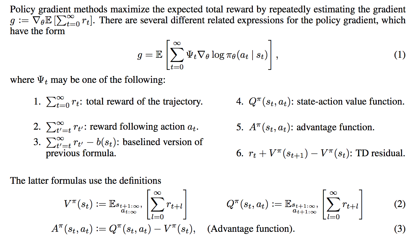
If the above is not 100% clear to you, I recommend reviewing the basics of policy gradients. I covered five of the six forms of the \(\Psi_t\) function in my last post; the exception is the temporal difference residual, but I will go over these later here.

Somewhat annoyingly, they use the infinite-horizon setting. I find it easier to think about the finite horizon case, and I will clarify if I’m assuming that.

Proposition 1: \(\gamma\)-Just Estimators.

One of the first things they prove is Proposition 1, regarding “\(\gamma\)-just” advantage estimators. (The word “just” seems like an odd choice here, but I’m not complaining.) Suppose \(\hat{A}_t(s_{0:\infty},a_{0:\infty})\) is an estimate of the advantage function. A \(\gamma\)-just estimator (of the advantage function) results in

This is for one time step \(t\). If we sum over all time steps, by linearity of expectation we get

In other words, we get an unbiased estimate of the discounted gradient. Note, however, that this discounted gradient is different from the gradient of the actual function we’re trying to optimize, since that was for the undiscounted rewards. The authors emphasize this in a footnote, saying that they’ve already introduced bias by even assuming the use of a discount factor. (I’m somewhat pleased at myself for catching this in advance.)

The proof for Proposition 1 is based on proving it for one time step \(t\), which is all that is needed. The resulting term with \(\hat{A}_t\) in it splits into two terms due to linearity of expectation, one with the \(Q_t\) function and another with the baseline. The second term is zero due to the baseline causing the expectation to zero, which I derived in my previous post in the finite-horizon case. (I’m not totally sure how to do this in the infinite horizon case, due to technicalities involving infinity.)

The first term is unfortunately a little more complicated. Let me use the finite horizon \(T\) for simplicity so that I can easily write out the definition. They argue in the proof that:

Most of this proceeds by definitions of expectations and then “pushing” integrals into their appropriate locations. Unfortunately, I am unable to figure out how they did step (i). Specifically, I don’t see how the integral over \(a_t\) somehow “moves past” the \(\nabla_\theta \log \pi_\theta(a_t|s_t)\) term. Perhaps there is some trickery with the law of iterated expectation due to conditionals? If anyone else knows why and is willing to explain with detailed math somewhere, I would really appreciate it.

For now, I will assume this proposition to be true. It is useful because if we are given the form of estimator \(\hat{A}_t\) of the advantage, we can immediately tell if it is an unbiased advantage estimator.

Advantage Function Estimators

Now assume we have some function \(V\) which attempts to approximate the true value function \(V^\pi\) (or \(V^{\pi,\gamma}\) in the undiscounted setting).

• Note I: \(V\) is not the true value function. It is only our estimate of it, so \(V_\phi(s_t) \approx V^\pi(s_t)\). I added in the \(\phi\) subscript to indicate that we use a function, such as a neural network, to approximate the value. The weights of the neural network are entirely specified by \(\phi\).

• Note II: we also have our policy \(\pi_\theta\) parameterized by parameters \(\theta\), again typically a neural network. For now, assume that \(\phi\) and \(\theta\) are separate parameters; the authors mention some enticing future work where one can share parameters and jointly optimize. The combination of \(\pi_{\theta}\) and \(V_{\phi}\) with a policy estimator and a value function estimator is known as the actor-critic model with the policy as the actor and the value function as the critic. (I don’t know why it’s called a “critic” because the value function acts more like an “assistant”.)

Using \(V\), we can derive a class of advantage function estimators as follows:

These take on the form of temporal difference estimators where we first estimate the sum of discounted rewards and then we subtract the value function estimate of it. If \(V = V^{\pi,\gamma}\), meaning that \(V\) is exact, then all of the above are unbiased estimates for the advantage function. In practice, this will not be the case, since we are not given the value function.

The tradeoff here is that the estimators \(\hat{A}_t^{(k)}\) with small \(k\) have low variance but high bias, whereas those with large \(k\) have low bias but high variance. Why? I think of it based on the number of terms. With small \(k\), we have fewer terms to sum over (which means low variance). However, the bias is relatively large because it does not make use of extra “exact” information with \(r_K\) for \(K > k\). Here’s another way to think of it as emphasized in the paper: \(V(s_t)\) is constant among the estimator class, so it does not affect the relative bias or variance among the estimators: differences arise entirely due to the \(k\)-step returns.

One might wonder, as I originally did, how to make use of the \(k\)-step returns in practice. In Q-learning, we have to update the parameters (or the \(Q(s,a)\) “table”) after each current reward, right? The key is to let the agent run for \(k\) steps, and then update the parameters based on the returns. The reason why we update parameters “immediately” in ordinary Q-learning is simply due to the definition of Q-learning. With longer returns, we have to keep the Q-values fixed until the agent has explored more. This is also emphasized in the A3C paper from DeepMind, where they talk about \(n\)-step Q-learning.

The Generalized Advantage Estimator

It might not be so clear which of these estimators above is the most useful. How can we compute the bias and variance?

It turns out that it’s better to use all of the estimators, in a clever way. First, define the temporal difference residual \(\delta_t^V = r_t + \gamma V(s_{t+1}) - V(s_t)\). Now, here’s how the Generalized Advantage Estimator \(\hat{A}_t^{GAE(\gamma,\lambda)}\) is defined:

To derive this, one simply expands the definitions and uses the geometric series formula. The result is interesting to interpret: the exponentially-decayed sum of residual terms.

The above describes the estimator \(GAE(\gamma, \lambda)\) for \(\lambda \in [0,1]\) where adjusting \(\lambda\) adjusts the bias-variance tradeoff. We usually have \({\rm Var}(GAE(\gamma, 1)) > {\rm Var}(GAE(\gamma, 0))\) due to the number of terms in the summation (more terms usually means higher variance), but the bias relationship is reversed. The other parameter, \(\gamma\), also adjusts the bias-variance tradeoff … but for the GAE analysis it seems like the \(\lambda\) part is more important. Admittedly, it’s a bit confusing why we need to have both \(\gamma\) and \(\lambda\) (after all, we can absorb them into one constant, right?) but as you can see, the constants serve different roles in the GAE formula.

To make a long story short, we can put the GAE in the policy gradient estimate and we’ve got our biased estimate (unless \(\lambda=1\)) of the discounted gradient, which again, is itself biased due to the discount. Will this work well in practice? Stay tuned …

Reward Shaping Interpretation

Reward shaping originated from a 1999 ICML paper, and refers to the technique of transforming the original reward function \(r\) into a new one \(\tilde{r}\) via the following transformation with \(\Phi: \mathcal{S} \to \mathbb{R}\) an arbitrary real-valued function on the state space:

Amazingly, it was shown that despite how \(\Phi\) is arbitrary, the reward shaping transformation results in the same optimal policy and optimal policy gradient, at least when the objective is to maximize discounted rewards \(\sum_{t=0}^\infty \gamma^t r(s_t,a_t,s_{t+1})\). I am not sure whether the same is true with the undiscounted case as they have here, but it seems like it should since we can set \(\gamma=1\).

The more important benefit for their purposes, it seems, is that this reward shaping leaves the advantage function invariant for any policy. The word “invariant” here means that if we computed the advantage function \(A^{\pi,\gamma}\) for a policy and a discount factor in some MDP, the transformed MDP would have some advantage function \(\tilde{A}^{\pi,\gamma}\), but we would have \(A^{\pi,\gamma} = \tilde{A}^{\pi,\gamma}\) (nice!). This follows because if we consider the discounted sum of rewards starting at state \(s_t\) in the transformed MDP, we get

“Hitting” the above values with expectations (as Michael I. Jordan would say it) and substituting appropriate values results in the desired \(\tilde{A}^{\pi,\gamma}(s_t,a_t) = A^{\pi,\gamma}(s_t,a_t)\) equality.

The connection between reward shaping and the GAE is the following: suppose we are trying to find a good policy gradient estimate for the transformed MDP. If we try to maximize the sum of \((\gamma \lambda)\)-discounted sum of (transformed) rewards and set \(\Phi = V\), we get precisely the GAE! With \(V\) here, we have \(\tilde{r}(s_t,a_t,s_{t+1}) = \delta_t^V\), the residual term defined earlier.

To analyze the tradeoffs with \(\gamma\) and \(\lambda\), they use a response function:

Why is this important? They state it clearly:

The response function lets us quantify the temporal credit assignment problem: long range dependencies between actions and rewards correspond to nonzero values of the response function for \(l \gg 0\).

These “long-range dependencies” are the most challenging part of the credit assignment problem. Then here’s the kicker: they argue that if \(\Phi = V^{\pi,\gamma}\), then the transformed rewards are such that \(\mathbb{E}[\tilde{r}_{l+t} \mid s_t,a_t] - \mathbb{E}[\tilde{r}_{l+t} \mid s_t] = 0\) for \(l>0\). Thus, long-range rewards have to induce an immediate response! I’m admittedly not totally sure if I understand this, and it seems odd that we only want the response function to be nonzero at the current time (I mean, some rewards have to be merely a few steps in the future, right?). I will take another look at this section if I have time.

Value Function Estimation

In order to be able to use the GAE in our policy gradient algorithm (again, this means computing gradients and shifting the weights of the policy to maximize an objective), we need some value function \(V_\phi\) parameterized by a neural network. This is part of the actor-critic framework, where the “critic” provides the value function estimate.

Let \(\hat{V}_t = \sum_{l=0}^\infty \gamma^l r_{t+l}\) be the discounted sum of rewards. The authors propose the following optimization procedure to find the best weights \(\phi\):

where each iteration, \(\phi_{\rm old}\) is the parameter vector before the update, and

This is a constrained optimization problem to find the best weights for the value function. The constraint reminds me of Trust Region Policy Optimization, because it limits the amount that \(\phi\) can change from one update to another. The advantages with a “trust region” method are that the weights don’t change too much and that they don’t overfit to the current batch. (Updates are done in batch mode, which is standard nowadays.)

• Note I: unfortunately, the authors don’t use this optimization procedure exactly. They use a conjugate gradient method to approximate it. But think of the optimization procedure here since it’s easier to understand and is “ideal.”

• Note II: remember that this is not the update to the policy \(\pi_\theta\). That update requires an entirely separate optimization procedure. Don’t get confused between the two. Both the policy and the value functions can be implemented as neural networks, and in fact, that’s what the authors do. They actually have the same architecture, with the exception of the output layer since the value only needs a scalar, whereas the policy needs a higher-dimensional output vector.

Putting it All Together

It’s nice to understand each of the components above, but how do we combine them into an actual algorithm? Here’s a rough description of their proposed actor-critic algorithm, each iteration:

• Simulate the current policy to collect data.

• Compute the Bellman residuals \(\delta_{t}^V\).

• Compute the advantage function estimate \(\hat{A}_t\).

• Update the policy’s weights, \(\theta_{i+1}\), with a TRPO update.

• Update the critic’s weights, \(\phi_{i+1}\), with a trust-region update.

As usual, here are a few of my overly-detailed comments (sorry again):

• Note I: Yes, there are trust region methods for both the value function update and the policy function update. This is one of their contributions. (To be clear, the notion of a “GAE” isn’t entirely their contribution.) The value and policy are also both neural networks with the same architecture except for the output since they have different outputs. Honestly, it seems like we should always be thinking about trust region methods whenever we have some optimization to do.

• Note II: If you’re confused by the role of the two networks, repeat this to yourself: the policy network is for determining actions, and the value network is for improving the performance of the gradient update (which is used to improve the actual policy by pointing the gradient in the correct direction!).

They present some impressive experimental benchmarks using this actor-critic algorithm. I don’t have too much experience with MuJoCo so I can’t intuitively think about the results that much. (I’m also surprised that MuJoCo isn’t free and requires payment; it must be by far the best physics simulator for reinforcement learning, otherwise people wouldn’t be using it.)

Concluding Thoughts

I didn’t understand the implications of this paper when I read it for the first time (maybe more than a year ago!) but it’s becoming clearer now. They present and analyze a specific kind of estimator, the GAE, which has a bias-variance “knob” with the \(\lambda\) (and \(\gamma\), technically). By adjusting the knob, it might be possible to get low variance, low biased estimates, which would drastically improve the sample efficiency of policy gradient methods. They also present a way to estimate the value method using a trust region method. With these components, they are able to achieve high performance on challenging reinforcement learning tasks with continuous control.