As I stated in my last blog post, I am feverishly trying to read more research papers. One category of papers that seems to be coming up a lot recently are those about policy gradients, which are a popular class of reinforcement learning algorithms which estimate a gradient for a function approximator. Thus, the purpose of this blog post is for me to explicitly write the mathematical foundations for policy gradients so that I can gain understanding. In turn, I hope some of my explanations will be useful to a broader audience of AI students.

Assumptions and Problem Statement

In any type of research domain, we always have to make some set of assumptions. (By “we”, I refer to the researchers who write papers on this.) With reinforcement learning and policy gradients, the assumptions usually mean the episodic setting where an agent engages in multiple trajectories in its environment. As an example, an agent could be playing a game of Pong, so one episode or trajectory consists of a full start-to-finish game.

We define a trajectory \(\tau\) of length \(T\) as

where \(s_0\) comes from the starting distribution of states, \(a_i \sim \pi_\theta(a_i| s_i)\), and \(s_i \sim P(s_i | s_{i-1},a_{i-1})\) with \(P\) the dynamics model (i.e. how the environment changes). We actually ignore the dynamics when optimizing, since all we care about is getting a good gradient signal for \(\pi_\theta\) to make it better. If this isn’t clear now, it will be clear soon. Also, the reward can be computed from the states and actions, since it’s usually a function of \((s_i,a_i,s_{i+1})\), so it’s not technically needed in the trajectory.

What’s our goal here with policy gradients? Unlike algorithms such as DQN, which strive to find an excellent policy indirectly through Q-values, policy gradients perform a direct gradient update on a policy to change its parameters, which is what makes it so appealing. Formally, we have:

• Note I: I put \(\pi_{\theta}\) under the expectation. This means the rewards are computed from a trajectory which was generated under the policy \(\pi_\theta\). We have to find “optimal” settings of \(\theta\) to make this work.

• Note II: we don’t need to optimize the expected sum of discounted rewards, though it’s the formulation I’m most used to. Alternatives include ignoring \(\gamma\) by setting it to one, extending \(T\) to infinity if the episodes are infinite-horizon, and so on.

The above raises the all-important question: how do we find the best \(\theta\)? If you’ve taken optimization classes before, you should know the answer already: perform gradient ascent on \(\theta\), so we have \(\theta \leftarrow \theta + \alpha \nabla f(x)\) where \(f(x)\) is the function being optimized. Here, that’s the expected value of whatever sum of rewards formula we’re using.

Two Steps: Log-Derivative Trick and Determining Log Probability

Before getting to the computation of the gradient, let’s first review two mathematical facts which will be used later, and which are also of independent interest. The first is the “log-derivative” trick, which tells us how to insert a log into an expectation when starting from \(\nabla_\theta \mathbb{E}[f(x)]\). Specifically, we have:

where \(p_\theta\) is the density of \(x\). Most of these steps should be straightforward. The main technical detail to worry about is exchanging the gradient with the integral. I have never been comfortable in knowing when we are allowed to do this or not, but since everyone else does this, I will follow them.

Another technical detail we will need is the gradient of the log probability of a trajectory since we will later switch \(x\) from above with a trajectory \(\tau\). The computation of \(\log p_\theta(\tau)\) proceeds as follows:

The probability of \(\tau\) decomposes into a chain of probabilities by the Markov Decision Process assumption, whereby the next action only depends on the current state, and the next state only depends on the current state and action. To be explicit, we use the functions that we already defined: \(\pi_\theta\) and \(P\) for the policy and dynamics, respectively. (Here, \(\mu\) represents the starting state distribution.) We also observe that when taking gradients, the dynamics disappear!

Computing the Raw Gradient

Using the two tools above, we can now get back to our original goal, which was to compute the gradient of the expected sum of (discounted) rewards. Formally, let \(R(\tau)\) be the reward function we want to optimize (i.e. maximize). Using the above two tricks, we obtain:

In the above, the expectation is with respect to the policy function, so think of it as \(\tau \sim \pi_\theta\). In practice, we need trajectories to get an empirical expectation, which estimates this actual expectation.

So that’s the gradient! Unfortunately, we’re not quite done yet. The naive way is to run the agent on a batch of episodes, get a set of trajectories (call it \(\hat{\tau}\)) and update with \(\theta \leftarrow \theta + \alpha \nabla_\theta \mathbb{E}_{\tau \in \hat{\tau}}[R(\tau)]\) using the empirical expectation, but this will be too slow and unreliable due to high variance on the gradient estimates. After one batch, we may exhibit a wide range of results: much better performance, equal performance, or worse performance. The high variance of these gradient estimates is precisely why there has been so much effort devoted to variance reduction techniques. (I should also add from personal research experience that variance reduction is certainly not limited to reinforcement learning; it also appears in many statistical projects which concern a bias-variance tradeoff.)

How to Introduce a Baseline

The standard way to reduce the variance of the above gradient estimates is to insert a baseline function \(b(s_t)\) inside the expectation.

For concreteness, assume \(R(\tau) = \sum_{t=0}^{T-1}r_t\), so we have no discounted rewards. We can express the policy gradient in three equivalent, but perhaps non-intuitive ways:

Comments:

• Step (i) follows from plugging in our chosen \(R(\tau)\) into the policy gradient we previously derived.

• Step (ii) follows from first noting that \(\nabla_\theta \mathbb{E}_{\tau}\Big[r_{t'}\Big] = \mathbb{E}_\tau\left[r_{t'} \cdot \sum_{t=0}^{t'} \nabla_\theta \log \pi_\theta(a_t|s_t)\right]\). The reason why this is true can be somewhat tricky to identify. I find it easy to think of just re-defining \(R(\tau)\) as \(r_{t'}\) for some fixed time-step \(t'\). Then, we do the exact same computation above to get the final result, as shown in the equation of the “Computing the Raw Gradient” section. The main difference now is that since we’re considering the reward at time \(t'\), our trajectory under expectation stops at that time. More concretely, \(\nabla_\theta\mathbb{E}_{(s_0,a_0,\ldots,s_{T})}\Big[r_{t'}\Big] = \nabla_\theta\mathbb{E}_{(s_0,a_0,\ldots,s_{t'})}\Big[r_{t'}\Big]\). This is like “throwing away variables” when taking expectations due to “pushing values” through sums and summing over densities (which cancel out); I have another example later in this post which makes this explicit.

  Next, we sum over both sides, for \(t' = 0,1,\ldots,T-1\). Assuming we can exchange the sum with the gradient, we get

  \[\begin{align} \nabla_\theta \mathbb{E}_{\tau \sim \pi_\theta} \left[ R(\tau) \right] &= \nabla_\theta \mathbb{E}_{\tau \sim \pi_\theta} \left[ \sum_{t'=0}^{T-1} r_{t'}\right] \\ &= \sum_{t'=0}^{T-1}\nabla_\theta \mathbb{E}_{\tau^{(t')}} \Big[r_{t'}\Big] \\ &= \sum_{t'}^{T-1} \mathbb{E}_{\tau^{(t')}}\left[r_{t'} \cdot \sum_{t=0}^{t'} \nabla_\theta \log \pi_\theta(a_t|s_t)\right] \\ &= \mathbb{E}_{\tau \sim \pi_\theta}\left[ \sum_{t'}^{T-1} r_{t'} \cdot \sum_{t=0}^{t'} \nabla_\theta \log \pi_\theta(a_t|s_t)\right]. \end{align}\]

  where \(\tau^{(t')}\) indicates the trajectory up to time \(t'\). (Full disclaimer: I’m not sure if this formalism with \(\tau\) is needed, and I think most people would do this computation without worrying about the precise expectation details.)

• Step (iii) follows from a nifty algebra trick. To simplify the subsequent notation, let \(f_t := \nabla_\theta \log \pi_\theta(a_t|s_t)\). In addition, ignore the expectation; we’ll only re-arrange the inside here. With this substitution and setup, the sum inside the expectation from Step (ii) turns out to be

  \[\begin{align} r_0f_0 &+ \\ r_1f_0 &+ r_1f_1 + \\ r_2f_0 &+ r_2f_1 + r_2f_2 + \\ \cdots \\ r_{T-1}f_0 &+ r_{T-1}f_1 + r_{T-1}f_2 \cdots + r_{T-1}f_{T-1} \end{align}\]

  In other words, each \(r_{t'}\) has its own row of \(f\)-value to which it gets distributed. Next, switch to the column view: instead of summing row-wise, sum column-wise. The first column is \(f_0 \cdot \left(\sum_{t=0}^{T-1}r_t\right)\). The second is \(f_1 \cdot \left(\sum_{t=1}^{T-1}r_t\right)\). And so on. Doing this means we get the desired formula after replacing \(f_t\) with its real meaning and hitting the expression with an expectation.

Note: it is very easy to make a typo with these. I checked my math carefully and cross-referenced it with references online (which themselves have typos). If any readers find a typo, please let me know.

Using the above formulation, we finally introduce our baseline \(b\), which is a function of \(s_t\) (and not \(s_{t'}\), I believe). We “insert” it inside the term in parentheses:

At first glance, it doesn’t seem like this will be helpful, and one might wonder if this would cause the gradient estimate to become biased. Fortunately, it turns out that this is not a problem. This was surprising to me, because all we know is that \(b(s_t)\) is a function of \(s_t\). However, this is a bit misleading because usually we want \(b(s_t)\) to be the expected return starting at time \(t\), which means it really “depends” on the subsequent time steps. For now, though, just think of it as a function of \(s_t\).

Understanding the Baseline

In this section, I first go over why inserting \(b\) above doesn’t make our gradient estimate biased. Next, I will go over why the baseline reduces variance of the gradient estimate. These two capture the best of both worlds: staying unbiased and reducing variance. In general, any time you have an unbiased estimate and it remains so after applying a variance reduction technique, then apply that variance reduction!

First, let’s show that the gradient estimate is unbiased. We see that with the baseline, we can distribute and rearrange and get:

Due to linearity of expectation, all we need to show is that for any single time \(t\), the gradient of \(\log \pi_\theta(a_t|s_t)\) multiplied with \(b(s_t)\) is zero. This is true because

Here are my usual overly-detailed comments (apologies in advance):

• Note I: this notation is similar to what I had before. The trajectory \(s_0,a_0,\ldots,a_{T-1},s_{T}\) is now represented as \(s_{0:T},a_{0:T-1}\). In addition, the expectation is split up, which is allowed. If this is confusing, think of the definition of the expectation with respect to at least two variables. We can write brackets in any appropriately enclosed location. Furthermore, we can “omit” the un-necessary variables in going from \(\mathbb{E}_{s_{t+1:T},a_{t:T-1}}\) to \(\mathbb{E}_{a_t}\) (see expression \(E\) above). Concretely, assuming we’re in discrete-land with actions in \(\mathcal{A}\) and states in \(\mathcal{S}\), this is because \(E\) evaluates to:

  \[\begin{align} E &= \sum_{a_t\in \mathcal{A}}\sum_{s_{t+1}\in \mathcal{S}}\cdots \sum_{s_T\in \mathcal{S}} \underbrace{\pi_\theta(a_t|s_t)P(s_{t+1}|s_t,a_t) \cdots P(s_T|s_{T-1},a_{T-1})}_{p((a_t,s_{t+1},a_{t+1}, \ldots, a_{T-1},s_{T}))} (\nabla_\theta \log \pi_\theta(a_t|s_t)) \\ &= \sum_{a_t\in \mathcal{A}} \pi_\theta(a_t|s_t)\nabla_\theta \log \pi_\theta(a_t|s_t) \sum_{s_{t+1}\in \mathcal{S}} P(s_{t+1}|s_t,a_t) \sum_{a_{t+1}\in \mathcal{A}}\cdots \sum_{s_T\in \mathcal{S}} P(s_T|s_{T-1},a_{T-1})\\ &= \sum_{a_t\in \mathcal{A}} \pi_\theta(a_t|s_t)\nabla_\theta \log \pi_\theta(a_t|s_t) \end{align}\]

  This is true because of the definition of expectation, whereby we get the joint density over the entire trajectory, and then we can split it up like we did earlier with the gradient of the log probability computation. We can distribute \(\nabla_\theta \log \pi_\theta(a_t|s_t)\) all the way back to (but not beyond) the first sum over \(a_t\). Pushing sums “further back” results in a bunch of sums over densities, each of which sums to one. The astute reader will notice that this is precisely what happens with variable elimination for graphical models. (The more technical reason why “pushing values back through sums” is allowed has to do with abstract algebra properties of the sum function, which is beyond the scope of this post.)

• Note II: This proof above also works with an infinite-time horizon. In Appendix B of the Generalized Advantage Estimation paper (arXiv link), the authors do so with a proof exactly matching the above, except that \(T\) and \(T-1\) are now infinity.

• Note III: About the expectation going to zero, that’s due to a well-known fact about score functions, which are precisely the gradient of log probailities. We went over this in my STAT 210A class last fall. It’s again the log derivative trick. Observe that:

  \[\mathbb{E}_{a_t}\Big[\nabla_\theta \log \pi_\theta(a_t|s_t)\Big] = \int \frac{\nabla_\theta \pi_\theta(a_t|s_t)}{\pi_{\theta}(a_t|s_t)}\pi_{\theta}(a_t|s_t)da_t = \nabla_\theta \int \pi_{\theta}(a_t|s_t)da_t = \nabla_\theta \cdot 1 = 0\]

  where the penultimate step follows from how \(\pi_\theta\) is a density. This follows for all time steps, and since the gradient of the log gets distributed for each \(t\), it applies in all time steps. I switched to the continuous-land version for this, but it also applies with sums, as I just recently used in Note I.

The above shows that introducing \(b\) doesn’t cause bias.

The last thing to cover is why its introduction reduces variance. I provide an approximate argument. To simplify notation, set \(R_t(\tau) = \sum_{t'=t}^{T-1}r_{t'}\). We focus on the inside of the expectation (of the gradient estimate) to analyze the variance. The technical reason for this is that expectations are technically constant (and thus have variance zero) but in practice we have to approximate the expectations with trajectories, and that has high variance.

The variance is approximated as:

Approximation (i) is because we are approximating the variance of a sum by computing the sum of the variances. This is not true in general, but if we can assume this, then by the definition of the variance \({\rm Var}(X) := \mathbb{E}[X^2]-(\mathbb{E}[X])^2\), we are left with the \(\mathbb{E}[X^2]\) term since we already showed that introducing the baseline doesn’t cause bias. Approximation (ii) is because we assume independence among the values involved in the expectation, and thus we can factor the expectation.

Finally, we are left with the term \(\mathbb{E}_{\tau} \left[\Big(R_t(\tau) - b(s_t))^2\right]\). If we are able to optimize our choice of \(b(s_t)\), then this is a least squares problem, and it is well known that the optimal choice of \(b(s_t)\) is to be the expected value of \(R_t(\tau)\). In fact, that’s why policy gradient researchers usually want \(b(s_t) \approx \mathbb{E}[R_t(\tau)]\) to approximate the expected return starting at time \(t\), and that’s why in the vanilla policy gradient algorithm we have to re-fit the baseline estimate each time to make it as close to the expected return \(\mathbb{E}[R_t(\tau)]\). At last, I understand.

How accurate are these approximations in practice? My intuition is that they are actually fine, because recent advances in reinforcement learning algorithms, such as A3C, focus on the problem of breaking correlation among samples. If the correlation among samples is broken, then Approximation (i) becomes better, because I think the samples \(s_0,a_0,\ldots,a_{T-1},s_{T}\) are no longer generated from the same trajectory.

Well, that’s my intuition. If anyone else has a better way of describing it, feel free to let me know in the comments or by email.

Discount Factors

So far, we have assumed we wanted to optimize the expected return, or the expected sum of rewards. However, if you’ve studied value iteration and policy iteration, you’ll remember that we usually use discount factors \(\gamma \in (0,1]\). These empirically work well because the effect of an action many time steps later is likely to be negligible compared to other action. Thus, it may not make sense to try and include raw distant rewards in our optimization problem. Thus, we often impose a discount as follows:

where the \(\gamma^{t'-t}\) serves as the discount, starting from 1, then getting smaller as time passes. (The first line above is a repeat of the policy gradient formula that I describe earlier.) As this is not exactly the “desired” gradient, this is an approximation, but it’s a reasonable one. This time, we now want our baseline to satisfy \(b(s_t) \approx \mathbb{E}[r_t + \gamma r_{t+1} + \cdots + \gamma^{T-1-t} r_{T-1}]\).

Advantage Functions

In this final section, we replace the policy gradient formula with the following value functions:

Both of these should be familiar from basic AI; see the CS 188 notes from Berkeley if this is unclear. There are also discounted versions, which we can denote as \(Q^{\pi,\gamma}(s,a)\) and \(V^{\pi,\gamma}(s)\). In addition, we can also consider starting at any given time step, as in \(Q^{\pi,\gamma}(s_t,a_t)\) which provides the expected (discounted) return assuming that at time \(t\), our state-action pair is \((s_t,a_t)\).

What might be new is the advantage function. For the undiscounted version, it is defined simply as:

with a similar definition for the discounted version. Intuitively, the advantage tells us how much better action \(a\) would be compared to the return based on an “average” action.

The above definitions look very close to what we have in our policy gradient formula. In fact, we can claim the following:

In (i), we replace terms with their expectations. This is not generally valid to do, but it should work in this case. My guess is that if you start from the second line above (after the “(i)”) and plug in the definition of the expectation inside and rearrange terms, you can get the first line. However, I have not had the time to check this in detail and it takes a lot of space to write out the expectation fully. The conditioning with the value functions makes it a bit messy and thus the law of iterated expectation may be needed.

Also from line (i), we notice that the value function is a baseline, and hence we can add it there without changing the unbiased-ness of the expectation. Then lines (ii) and (iii) are just for the advantage function. The implication of this formula is that the problem of policy gradients, in some sense, reduces to finding good estimates \(\hat{A}^{\pi,\gamma}(s_t,a_t)\) of the advantage function \(A^{\pi,\gamma}(s_t,a_t)\). That is precisely the topic of the paper Generalized Advantage Estimation.

Concluding Remarks

Hopefully, this is a helpful, self-contained, bare-minimum introduction to policy gradients. I am trying to learn more about these algorithms, and going through the math details is helpful. This will also make it easier for me to understand the increasing number of research papers that are using this notation.

I also have to mention: I remember a few years ago during the first iteration of CS 294-112 that I had no idea how policy gradients worked. Now, I think I have become slightly more enlightened.

Acknowledgements: I thank John Schulman for making his notes publicly available.

Update April 19, 2017: I have code for vanilla policy gradients in my reinforcement learning GitHub repository.

The number of research papers in Artificial Intelligence has reached un-manageable proportions. Conferences such as ICML, NIPS, and ICLR others are getting record amounts of paper submissions. In addition, tens of AI-related papers get uploaded to arXiv every weekday. With all these papers, it can be easy to feel lost and overwhelmed.

Like many researchers, I think I do not read enough research papers. This year, I resolved to change that, so I started an open-source GitHub repository called “Paper Notes” where I list papers that I’ve read along with my personal notes and summaries, if any. Papers without such notes are currently on my TODO radar.

After almost three months, I’m somewhat pleased with my reading progress. There are a healthy number of papers (plus notes) listed, arranged by subject matter and then further arranged by year. Not enough for me, but certainly not terrible either.

I was inspired to make this by seeing Denny Britz’s similar repository, along with Adrian Colyer’s blog. My repository is similar to Britz’s, though my aim is not to list all papers in Deep Learning, but to write down the ones that I actually plan to read at some point. (I see other repositories where people simply list Deep Learning papers without notes, which seems pretty pointless to me.) Colyer’s blog posts represent the kind of notes that I’d like to take for each paper, but I know that I can’t dedicate that much time to fine-tuning notes.

Why did I choose GitHub as the backend for my paper management, rather than something like Mendeley? First, GitHub is the default place where (pretty much) everyone in AI puts their open-source stuff: blogs, code, you name it. I’m already used to GitHub, so Mendeley would have to provide some serious benefit for me to switch over. I also don’t need to use advanced annotation and organizing materials, given that the top papers are easily searchable online (including their BibTeX references). In addition, by making my Paper Notes repository online, I can show this as evidence to others that I’m reading papers. Maybe this will even impress a few folks, and I say this only because everyone wants to be noticed in some way; that’s partly Colyer’s inspiration for his blog. So I think, on balance, it will be useful for me to keep updating this repository.

Update December 29, 2021: I now don’t use this repository very much, if at all. Instead, since I got an iPad two years ago, I’ve started to rely a lot on Notability which lets me download and annotate PDFs with the iPad pen. So far this is a slightly easier system for me to track papers that I read. However, I will keep the GitHub repository available in case it is of use to readers.

There’s an opinion piece in the New York Times by Moises Velasquez-Manoff which talks about (drum roll please) biracial people. As he mentions:

Multiracials make up an estimated 7 percent of Americans, according to the Pew Research Center, and they’re predicted to grow to 20 percent by 2050.

Thus, I suspect that sometime in the next few decades, we will start talking about race in terms of precise racial percentages, such as “100 percent White” or in rarer cases, “25 percent White, 25 percent Asian, 25 percent Black, and 25 percent Native American.” (Incidentally, I’m not sure why the article uses “Biracial” when “Multiracial” would clearly have been a more appropriate term; it was likely due to the Barack Obama factor.)

The phrase “precise racial percentages” is misleading. Since all humans came from the same ancestor, at some point in history we must have been “one race.” For the sake of defining these racial percentages, we can take a date — say 4000BC — when, presumably, the various races were sufficiently different, ensconced in their respective geographic regions, and when interracial marriages (or rape) was at a minimum. All humans alive at that point thus get a “100 percent [insert_race_here]” attached to them, and we do the arithmetic from there.

What usually happens in practice, though, is that we often default to describing one part of one race, particularly with people who are \(X\) percent Black, where \(X > 0\). This is a relic of the embarrassing “One Drop Rule” the United States had, but for now it’s probably — well, I hope — more for self-selecting racial identity.

Listing precise racial percentages would help us better identify people who are not easy to immediately peg in racial categories, which will increasingly become an issue as more and more multiracial people like me blur the lines between the races. In fact, this is already a problem for me even with single-race people: I sometimes cannot distinguish between Hispanics versus Whites. For instance, I thought Ted Cruz and Marco Rubio were 100 percent White.

Understanding race is also important when considering racial diversity and various ethical or sensitive questions over who should get “preferences.” For instance, I wonder if people label me as a “privileged white male” or if I get a pass for being biracial? Another question: for a job at a firm which has had a history of racial discrimination and is trying to make up for that, should the applicant who is 75 percent Black, 25 percent White, get a hair’s preference versus someone who is 25 percent Black and 75 percent White? Would this also apply if they actually have very similar skin color?

In other words, does one weigh more towards the looks or the precise percentages? I think the precise percentages method is the way schools, businesses, and government operate, despite how this isn’t the case in casual conversations.

Anyway, these are some of the thoughts that I have as we move towards a more racially diverse society, as multiracial people cannot have single-race children outside of adoption.

Back to the article: as one would expect, it discusses the benefits of racial diversity. I can agree with the following passage:

Social scientists find that homogeneous groups like [Donald Trump’s] cabinet can be less creative and insightful than diverse ones. They are more prone to groupthink and less likely to question faulty assumptions.

The caveat is that this assumes the people involved are equally qualified; a racially homogeneous (in whatever race), but extremely well-educated cabinet would be much better than a racially diverse cabinet where no one even finished high school. But controlling for quality, I can agree.

Diversity also benefits individuals, as the author notes. It is here where Mr. Velasquez-Manoff points out that Barack Obama was not just Black, but also biracial, which may have benefited his personal development. Multiracials make up a large fraction of the population in racially diverse Hawaii, where Obama was born (albeit, probably with more Asian-White overlap).

Yes, I agree that diversity is important for a variety of reasons. It is not easy, however:

It’s hard to know what to do about this except to acknowledge that diversity isn’t easy. It’s uncomfortable. It can make people feel threatened. “We promote diversity. We believe in diversity. But diversity is hard,” Sophie Trawalter, a psychologist at the University of Virginia, told me.

That very difficulty, though, may be why diversity is so good for us. “The pain associated with diversity can be thought of as the pain of exercise,” Katherine Phillips, a senior vice dean at Columbia Business School, writes. “You have to push yourself to grow your muscles.”

I cannot agree more.

Moving on:

Closer, more meaningful contact with those of other races may help assuage the underlying anxiety. Some years back, Dr. Gaither of Duke ran an intriguing study in which incoming white college students were paired with either same-race or different-race roommates. After four months, roommates who lived with different races had a more diverse group of friends and considered diversity more important, compared with those with same-race roommates. After six months, they were less anxious and more pleasant in interracial interactions.

Ouch, this felt like a blindsiding attack, and is definitely my main gripe with this article. In college, I had two roommates, both of whom have a different racial makeup than me. They both seemed to be relatively popular and had little difficulty mingling with a diverse group of students. Unfortunately, I certainly did not have a “diverse group of friends.” After all, if there was a prize for college for “least popular student” I would be a perennial contender. (As incredible as it may sound, in high school, where things were worse for me, I can remember a handful of people who might have been even lower on the social hierarchy.)

Well, I guess what I want to say is that, this attack notwithstanding, Mr. Velasquez-Manoff’s article brings up interesting and reasonably accurate points about biracial people. At the very least, he writes about concepts which are sometimes glossed over or under-appreciated nowadays in our discussions about race.

Over the last few weeks, I’ve been learning more about some mysterious thing called Generative Adversarial Networks (GANs). GANs originally came out of a 2014 NIPS paper (read it here) and have had a remarkable impact on machine learning. I’m surprised that, until I was the TA for Berkeley’s Deep Learning class last semester, I had never heard of GANs before.¹

They certainly haven’t gone unnoticed in the machine learning community, though. Yann LeCun, one of the leaders in the Deep Learning community, had this to say about them during his Quora session on July 28, 2016:

The most important one, in my opinion, is adversarial training (also called GAN for Generative Adversarial Networks). This is an idea that was originally proposed by Ian Goodfellow when he was a student with Yoshua Bengio at the University of Montreal (he since moved to Google Brain and recently to OpenAI).

This, and the variations that are now being proposed is the most interesting idea in the last 10 years in ML, in my opinion.

If he says something like that about GANs, then I have no excuse for not learning about them. Thus, I read what is probably the highest-quality general overview available nowadays: Ian Goodfellow’s tutorial on arXiv, which he then presented in some form at NIPS 2016. This was really helpful for me, and I hope that later, I can write something like this (but on another topic in AI).

I won’t repeat what GANs can do here. Rather, I’m more interested in knowing how GANs are trained. Following now are some of the most important insights I gained from reading the tutorial:

• Major Insight 1: the discriminator’s loss function is the cross entropy loss function. To understand this, let’s suppose we’re doing some binary classification with some trainable function \(D: \mathbb{R}^n \to [0,1]\) that we wish to optimize, where \(D\) indicates the estimated probability of some data point \(x_i \in \mathbb{R}^n\) being in the first class. To get the predicted probability of being in the second class, we just do \(1-D(x_i)\). The output of \(D\) must therefore be constrained in \([0,1]\), which is easy to do if we tack on a sigmoid layer at the end. Furthermore, let \((x_i,y_i) \in (\mathbb{R}^n, \{0,1\})\) be the input-label pairing for training data points.

  The cross entropy between two distributions, which we’ll call \(p\) and \(q\), is defined as

  \[H(p,q) := -\sum_i p_i \log q_i\]

  where \(p\) and \(q\) denote a “true” and an “empirical/estimated” distribution, respectively. Both are discrete distributions, hence we can sum over their individual components, denoted with \(i\). (We would need to have an integral instead of a sum if they were continuous.) Above, when I refer to a “distribution,” it means with respect to a single training data point, and not the “distribution of training data points.” That’s a different concept.

  To apply this loss function to the current binary classification task, for (again) a single data point \((x_i,y_i)\), we define its “true” distribution as \(\mathbb{P}[y_i = 0] = 1\) if \(y_i=0\), or \(\mathbb{P}[y_i = 1] = 1\) if \(y_i=1\). Putting in 2-D vector form, it’s either \([1,0]\) or \([0,1]\). Intuitively, we know for sure which class this belongs to (because it’s part of the training data), so it makes sense for a probability distribution to be a “one-hot” vector.

  Thus, for one data point \(x_1\) and its label, we get the following loss function, where here I’ve changed the input to be more precise:

  \[H((x_1,y_1),D) = - y_1 \log D(x_1) - (1-y_1) \log (1-D(x_1))\]

  Let’s look at the above function. Notice that only one of the two terms is going to be zero, depending on the value of \(y_1\), which makes sense since it’s defining a distribution which is either \([0,1]\) or \([1,0]\). The other part is the estimated distribution from \(D\). In both cases (the true and predicted distributions) we are encoding a 2-D distribution with one value, which lets us treat \(D\) as a real-valued function.

  That was for one data point. Summing over the entire dataset of \(N\) elements, we get something that looks like this:

  \[H((x_i,y_i)_{i=1}^N,D) = - \sum_{i=1}^N y_i \log D(x_i) - \sum_{i=1}^N (1-y_i) \log (1-D(x_i))\]

  In the case of GANs, we can say a little more about what these terms mean. In particular, our \(x_i\)s only come from two sources: either \(x_i \sim p_{\rm data}\), the true data distribution, or \(x_i = G(z)\) where \(z \sim p_{\rm generator}\), the generator’s distribution, based on some input code \(z\). It might be \(z \sim {\rm Unif}[0,1]\) but we will leave it unspecified.

  In addition, we also want exactly half of the data to come from these two sources.

  To apply this to the sum above, we need to encode this probabilistically, so we replace the sums with expectations, the \(y_i\) labels with \(1/2\), and we can furthermore replace the \(\log (1-D(x_i))\) term with \(\log (1-D(G(z)))\) under some sampled code \(z\) for the generator. We get

  \[H((x_i,y_i)_{i=1}^\infty,D) = - \frac{1}{2} \mathbb{E}_{x \sim p_{\rm data}}\Big[ \log D(x)\Big] - \frac{1}{2} \mathbb{E}_{z} \Big[\log (1-D(G(z)))\Big]\]

  This is precisely the loss function for the discriminator, \(J^{(J)}\).

• Major Insight 2: understanding how gradient saturation may or may not adversely affect training. Gradient saturation is a general problem when gradients are too small (i.e. zero) to perform any learning. See Stanford’s CS 231n notes on gradient saturation here for more details. In the context of GANs, gradient saturation may happen due to poor design of the generator’s loss function, so this “major insight” of mine is also based on understanding the tradeoffs among different loss functions for the generator. This design, incidentally, is where we can be creative; the discriminator needs the cross entropy loss function above since it has a very specific function (to discriminate among two classes) and the cross entropy is the “best” way of doing this.

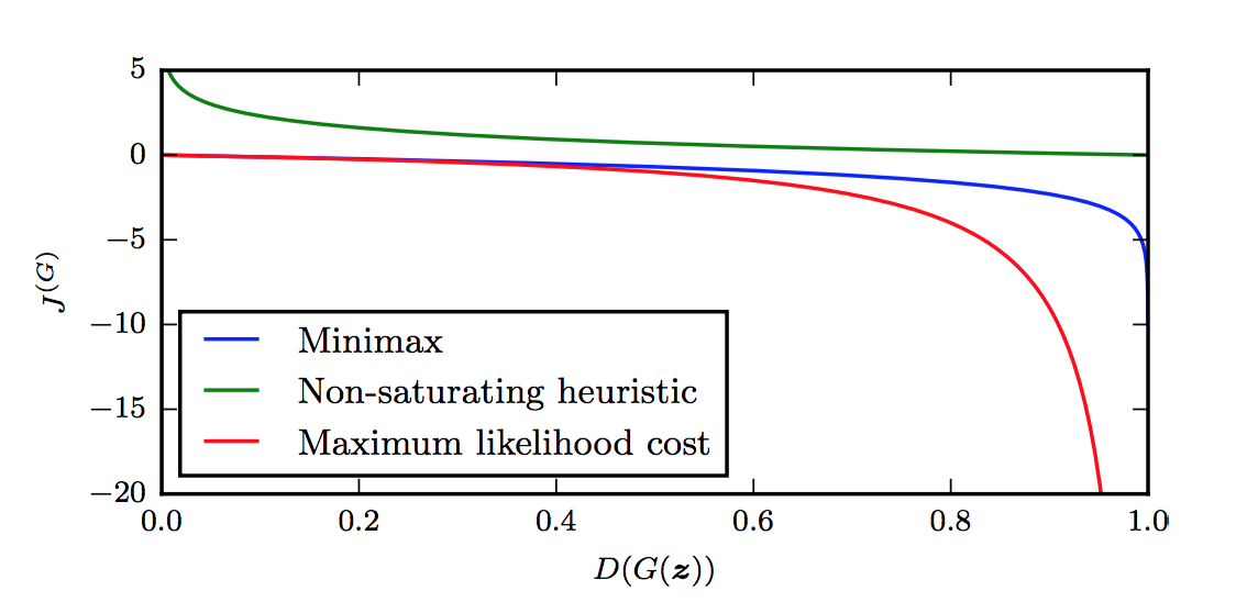
  Using Goodfellow’s notation, we have the following candidates for the generator loss function, as discussed in the tutorial. The first is the minimax version:

  \[J^{(G)} = -J^{(J)} = \frac{1}{2} \mathbb{E}_{x \sim p_{\rm data}}\Big[ \log D(x)\Big] + \frac{1}{2} \mathbb{E}_{z} \Big[\log (1-D(G(z)))\Big]\]

  The second is the heuristic, non-saturating version:

  \[J^{(G)} = -\frac{1}{2}\mathbb{E}_z\Big[\log D(G(z))\Big]\]

  Finally, the third is the maximum likelihood version:

  \[J^{(G)} = -\frac{1}{2}\mathbb{E}_z\left[e^{\sigma^{-1}(D(G(z)))}\right]\]

  What are the advantages and disadvantages of these generator loss functions? For the minimax version, it’s simple and allows for easier theoretical results, but in practice its not that useful, due to gradient saturation. As Goodfellow notes:

  In the minimax game, the discriminator minimizes a cross-entropy, but the generator maximizes the same cross-entropy. This is unfortunate for the generator, because when the discriminator successfully rejects generator samples with high confidence, the generator’s gradient vanishes.

  As suggested in Chapter 3 of Michael Nielsen’s excellent online book, the cross-entropy is a great loss function since it is designed in part to accelerate learning and avoid gradient saturation only up to when the classifier is correct (since we don’t want the gradient to move in that case!).

  I’m not sure how to clearly describe this formally. For now, I will defer to Figure 16 in Goodfellow’s tutorial (see the top of this blog post), which nicely shows the value of \(J^{(G)}\) as a function of the discriminator’s output, \(D(G(z))\). Indeed, when the discriminator is winning, we’re at the left side of the graph, since the discriminator outputs the probability of the sample being from the true data distribution.

  By the way, why is \(J^{(G)} = -J^{(J)}\) only a function of \(D(G(z))\) as suggested by the figure? What about the other term in \(J^{(J)}\)? Notice that of the two terms in the loss function, the first one is only a function of the discriminator’s parameters! The second part, which uses the \(D(G(z))\) term, depends on both \(D\) and \(G\). Hence, for the purposes of performing gradient descent with respect to the parameters of \(G\), only the second term in \(J^{(J)}\) matters; the first term is a constant that disappears after taking derivatives \(\nabla_{\theta^{(G)}}\).

  The figure makes it clear that the generator will have a hard time doing any sort of gradient update at the left portion of the graph, since the derivatives are close to zero. The problem is that the left portion of the graph represents the most common case when starting the game. The generator, after all, starts out with basically random parameters, so the discriminator can easily tell what is real and what is fake.²

  Let’s move on to the other two generator cost functions. The second one, the heuristically-motivated one, uses the idea that the generator’s gradient only depends on the second term in \(J^{(J)}\). Instead of flipping the sign of \(J^{(J)}\), they instead flip the target: changing \(\log (1-D(G(z)))\) to \(\log D(G(z))\). In other words, the “sign flipping” happens at a different part, so the generator still optimizes something “opposite” of the discriminator. From this re-formulation, it appears from the figure above that \(J^{(G)}\) now has desirable gradients in the left portion of the graph. Thus, the advantage here is that the generator gets a strong gradient signal so that it can quickly improve. The downside is that it’s not easier to analyze, but who cares?

  Finally, the maximum likelihood cost function has the advantage of being motivated based on maximum likelihood, which by itself has a lot of desirable properties. Unfortunately, the figure above shows that it has a flat slope in the left portion, though it seems to be slightly better than the minimax version since it decreases rapidly “sooner.” Though that might not be an “advantage,” since Goodfellow warns about high variance. That might be worth thinking about in more detail.

  One last note: the function \(J^{(G)}\), at least for the three cost functions here, does not depend directly on \(x\) at all! That’s interesting … and in fact, Goodfellow argues that makes GANs resistant to overfitting since it can’t copy from \(x\).

I wish more tutorials like this existed for other AI concepts. I particularly enjoyed the three exercises and the solutions within this tutorial on GANs. I have more detailed notes here in my Paper Notes GitHub repository (I should have started this repository back in 2013). I highly recommend this tutorial to anyone wanting to know more about GANs.

Update March 26, 2020: made a few clarifications.

CS 231n: Convolutional Neural Networks for Visual Recognition is, in my biased opinion, one of the most important and thrilling courses offered by Stanford University. It has been taught twice so far and will appear again in the upcoming Spring quarter.

Due to its popularity, the course lectures for the second edition (Winter 2016) were videotaped and released online. This is not unusual among computer science graduate level courses due to high demand both inside and outside the university.

Unfortunately, as discussed in this rather large reddit discussion thread, Andrej Karpathy (one of the three instructors) was forced to pull down the lecture videos. He later clarified on his Twitter account that the reason had to do with the lack of captioning/subtitles in the lecture videos, which relates to a news topic I blogged about just over two years ago.

If you browse the reddit thread, you will see quite a lot of unhappy students. I just joined reddit and I was hoping to make a comment there, but reddit disables posting after six months. And after thinking about it, I thought it would make more sense to write some brief thoughts here instead.

To start, I should state upfront that I have no idea what happened beyond the stuff we can all read online. I don’t know who made the complaint, what the course staff did, etc.

Here’s my stance regarding class policies on watching videos:

If a class requires watching videos for whatever reason, then that video should have subtitles. Otherwise, no such action is necessary, though the course staff should attempt as much as is reasonable to have subtitles for all videos.

I remember two times when I had to face this problem of watching a non-subtitled video as a homework assignment: in an introductory Women’s, Gender, and Sexuality Studies course and an Africana Studies class about black athletes. For the former, we were assigned to watch a video about a transgender couple, and for the latter, the video was about black golfers. In both cases, the professors gave me copies of the movie (other students didn’t get these) and I watched one in a room myself with the volume cranked up and the other one with another person who told me what was happening.

Is that ideal? Well, no. To (new) readers of this blog, welcome to the story of my life!

More seriously, was I supposed to do something about it? The professors didn’t make the videos, which were a tiny portion of the overall courses. I didn’t want to get all up in arms about this, so in both cases, I brought it up with them and they understood my situation (and apologized).

Admittedly, my brief stance above is incomplete and belies a vast gray area. What if students are given the option of doing one of two “required” assignments: watching a video or reading a book? That’s a gray area, though I would personally lean that towards “required viewing” and thus “required subtitles.”

Class lecture videos also fall in a gray area. They are not required viewing, because students should attend lectures in person. Unfortunately, the lack of subtitles for these videos definitely puts deaf and hard of hearing students like myself at a disadvantage. I’ve lost count of the amount of lectures that I wish I could have re-watched, but it extraordinarily difficult for me to do so for non-subtitled videos.

Ultimately, however, as long as I can attend lectures and understand some of the material, I do not worry about whether lecture videos have subtitles. Just about every videotaped class that I have taken did not have subtitled lecture videos, with one exception: CS 267 from Spring 2016, after I had negotiated about it with Berkeley’s DSP.

Heck, the CS 294-129 class which I TA-ed for last semester — which is based on CS 231n! — had lecture videos. Were there captions? Nope.

Am I frustrated? Yes, but it’s understandable frustration due to the cost of adding subtitles. As a similar example, I’m frustrated at the identity politics practiced by the Democratic party, but it’s understandable frustration due to what political science instructs us to do, which is why I’m not planning to jump ship to another party.

Thus in my case, if I were a student in CS 231n, I would not be inclined to pressure the staff to pull the videos down. Again, this comes with the obvious caveat; I don’t know the situation and it might have been worse than I imagine.

As this discussion would imply, I don’t like pulling down lecture videos as “collateral damage”.¹ I worry, however, if that’s in part because I’m too timid. Hypothetically and broadly speaking, if I have to take out my frustration (e.g. with lawsuits) on certain things, I don’t want to do this for something like lecture videos, which would make a number of folks angry at me, whether or not they openly express it.

On a more positive note … it turns out that, actually, the CS 231n lecture videos are online! I’m not sure why, but I’m happy. Using YouTube’s automatic captions, I watched one of the lectures and finally understood a concept that was critical and essential for me to know when I was writing my latest technical blog post.

Moreover, the automatic captions are getting better and better each year. They work pretty well on Andrej, who has a slight accent (Russian?). I dislike attending research talks if I don’t understand what’s going on, but given that so many are videotaped these days, whether at Berkeley or at conferences, maybe watching them offline is finally becoming a viable alternative.

I am now wearing Oticon Dynamo hearing aids. The good news is that I’ve run many times with them and so far have not had issues with water resistance.

However, I wanted to bring up a striking point that really made me realize about how our world has changed remarkably in the last few years.

A few months ago, when I was first fitted with the hearing aids, my audiologist set the default volume level to be “on target” for me. The hearing aid is designed to provide different amounts of power to people depending on their raw hearing level. There’s a volume control on it which goes from “1” (weak) to “4” (powerful), which I can easily adjust as I wish. The baseline setting is “3”, but this baseline is what audiologist adjust on a case-by-case basis. This means my “3” (and thus, my “1” and “4” settings) may be more powerful, less powerful, or the same compared to the respective settings for someone else.

When my audiologist first fit the hearing aids for me, I felt that my left hearing aid was too quiet and my right one too loud by default, so she modified the baselines.

She also, critically, gave me about a week to adjust to the hearing aids, and I was to report back on whether its strength was correctly set.

During that week, I wore the hearing aids, but I then decided that I was originally mistaken about both hearing aids, since I had to repeatedly increase the volume for the left one and decrease the volume for the right one.

I reported back to my audiologist and said that she was right all along, and that my baselines needed to be back to their default levels. She was able to corroborate my intuition by showing me — amazingly – how often I had adjusted the hearing aid volume level, and in which direction.

Hearing aids are, apparently, now fitted with these advanced sensors so they can track exactly how you adjust them (volume controls or otherwise).

The lesson is that just about everything nowadays consists of sensors, a point which is highlighted in Thomas L. Friedman’s excellent book Thank You for Being Late. It is also a characteristic of what computer scientists refer to as the “Internet of Things.”

Obviously, these certainly aren’t the hearing aids your father wore when he was young.

I just signed a petition, Academics Against Immigration Executive Order to oppose the Trump administration’s recent executive order. You can find the full text here along with the names of those who have signed up. (Graduate students are in the “Other Signatories” category and may take a while to update.) I like this petition because it clearly lists the names of people so as to avoid claims of duplication and/or bogus signatures for anonymous petitions. There are lots of academic superstars on the list, including (I’m proud to say) my current statistics professor Michael I. Jordan and my statistics professor William Fithian from last semester.

The petition lists three compelling reasons to oppose the order, but let me just chime in with some extra thoughts.

I understand the need to keep our country safe. But in order to do so, there has to be a correct tradeoff in terms of security versus profiling (for lack of a better word) and in terms of costs versus benefits.

On the spectrum of security, to one end are those who deny the existence of radical Islam and the impact of religion on terrorism. On the other end are those who would happily ban an entire religion and place the blame and burden on millions of law-abiding people fleeing oppression. This order is far too close to the second end.

In terms of costs and benefits, I find an analogy to policing useful. Mayors and police chiefs shouldn’t be assigning their police officers uniformly throughout cities. The police should be targeted in certain hotspots of crime as indicated by past trends. That’s the most logical and cost-effective way to crack down on crime.

Likewise, if were are serious about stopping radical Islamic terrorism, putting a blanket ban on Muslims is like the “uniform policing strategy” and will also cause additional problems since Muslims would (understandably!) feel unfairly targeted. For instance, Iran is already promising “proportional responses”. I also have to mention that the odds of being killed by a refugee terrorist are so low that the amount of anxiety towards them does not justify the cost.

By the way, I’m still waiting for when Saudi Arabia — the source of 15 out of 19 terrorists responsible for 9/11 — gets on the executive order list. I guess President Trump has business dealings there? (Needless to say, that’s why conflict of interest laws exist.)

I encourage American academics to take a look at this order and (hopefully) sign the petition. I also urge our Secretary of Defense, James Mattis, to talk to Trump and get him to rescind and substantially revise the order. While I didn’t state this publicly to anyone, I have more respect for Mattis than any one else in the Trump cabinet, and hopefully that will remain the case.

Introduction

One of the major difficulties in understanding how neural networks work is due to the backpropagation algorithm. There are endless texts and online guides on backpropagation, but most are useless. I read several explanations of backpropagation when I learned about it from 2013 to 2014, but I never felt like I really understood it until I took/TA-ed the Deep Neural Networks class at Berkeley, based on the excellent Stanford CS 231n course.

The course notes from CS 231n include a tutorial on how to compute gradients for local nodes in computational graphs, which I think is key to understanding backpropagation. However, the notes are mostly for the one-dimensional case, and their main advice for extending gradient computation to the vector or matrix case is to keep track of dimensions. That’s perfectly fine, and in fact that was how I managed to get through the second CS 231n assignment.

But this felt unsatisfying.

For some of the harder gradient computations, I had to test several different ideas before passing the gradient checker, and sometimes I wasn’t even sure why my code worked! Thus, the purpose of this post is to make sure I deeply understand how gradient computation works.

Note: I’ve had this post in draft stage for a long time. However, I just found out that the notes from CS 231n have been updated with a guide from Erik Learned-Miller on taking matrix/vector derivatives. That’s worth checking out, but fortunately, the content I provide here is mostly distinct from his material.

The Basics: Computational Graphs in One Dimension

I won’t belabor the details on one-dimensional graphs since I assume the reader has read the corresponding Stanford CS 231n guide. Another nice post is from Chris Olah’s excellent blog. For my own benefit, I reviewed derivatives on computational graphs by going through the CS 231n example with sigmoids (but with the sigmoid computation spread out among finer-grained operations). You can see my hand-written computations in the following image. Sorry, I have absolutely no skill in getting this up quickly using tikz, Inkscape, or other visualization tactics/software. Feel free to right-click and open the image in a new tab. Warning: it’s big. (But I have to say, the iPhone7 plus makes really nice images. I remember the good old days when we had to take our cameras to CVS to get them developed…)

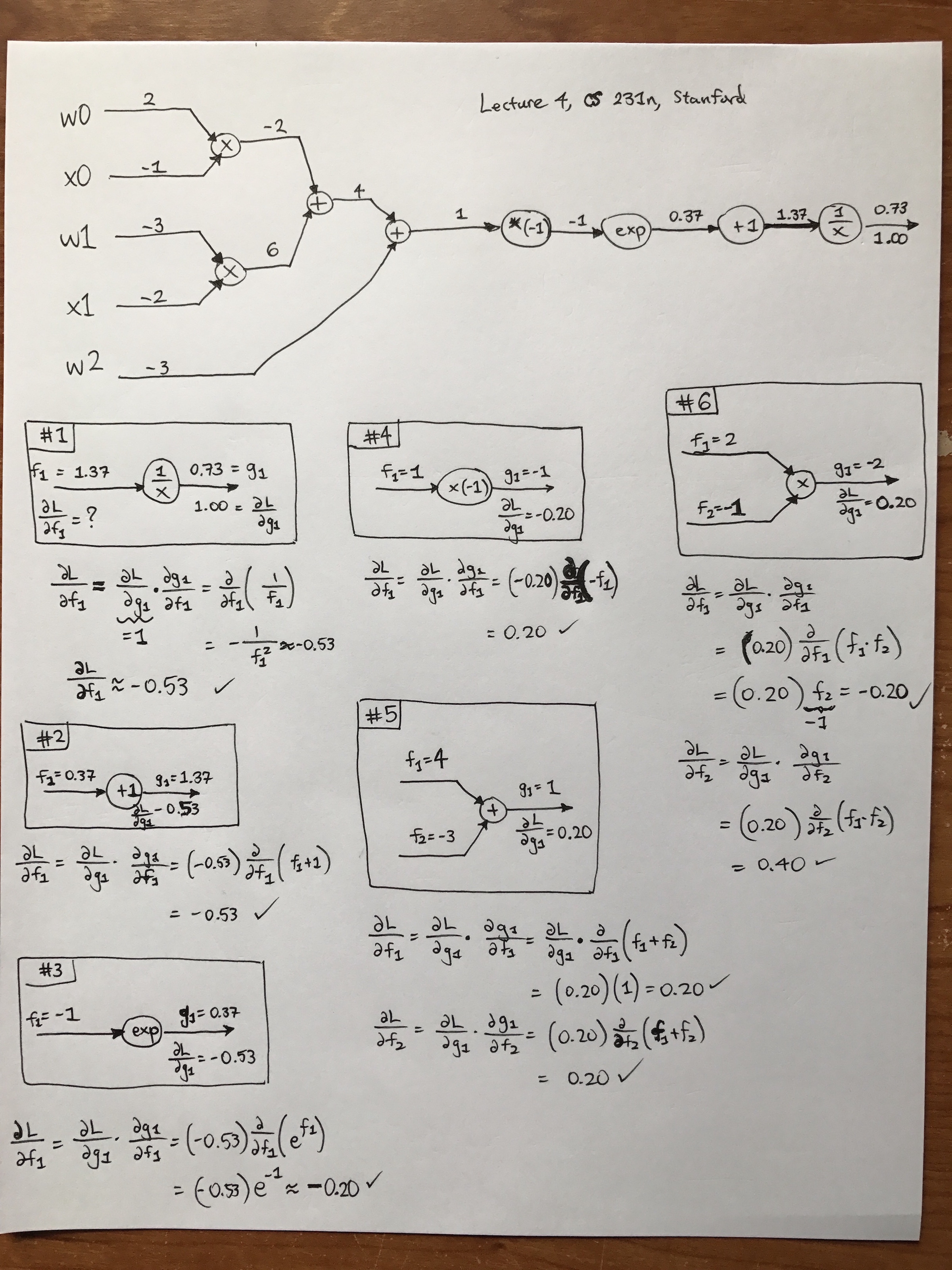
Another note: from the image, you can see that this is from the fourth lecture of CS 231n class. I watched that video on YouTube, which is excellent and of high-quality. Fortunately, there are also automatic captions which are highly accurate. (There’s an archived reddit thread discussing how Andrej Karpathy had to take down the videos due to a related lawsuit I blogged about earlier, but I can see them just fine. Did they get back up somehow? I’ll write more about this at a later date.)

When I was going through the math here, I came up with several rules to myself:

1. There’s a lot of notation that can get confusing, so for simplicity, I always denoted inputs as \(f_1,f_2,\ldots\) and outputs as \(g_1,g_2,\ldots\), though in this example, we only have one output at each step. By doing this, I can view the \(g_1\)s as a function of the \(f_i\) terms, so the local gradient turns into \(\frac{\partial g_1}{\partial f_i}\) and then I can substitute \(g_1\) in terms of the inputs.

2. When doing backpropgation, I analyzed it node-by-node, and the boxes I drew in my image contain a number which indicates the order I evaluated them. (I skipped a few repeat blocks just as the lecture did.) Note that when filling in my boxes, I only used the node and any incoming/outgoing arrows. Also, the \(f_i\) and \(g_i\) keep getting repeated, i.e. the next step will have \(g_i\) equal to whatever the \(f_i\) was in the previous block.

3. Always remember that when we have arrows here, the part above the arrow contains the value of \(f_i\) (respectively, \(g_i\)) and below the arrow we have \(\frac{\partial L}{\partial f_i}\) (respectively \(\frac{\partial L}{\partial g_i}\)).

Hopefully this will be helpful to beginners using computational graphs.

Vector/Matrix/Tensor Derivatives, With Examples

Now let’s get to the big guns — vectors/matrices/tensors. Vectors are a special case of matrices, which are a special case of tensors, the most generalized \(n\)-dimensional array. For this section, I will continue using the “partial derivative” notation \(\frac{\partial}{\partial x}\) to represent any derivative form (scalar, vector, or matrix).

ReLU

Our first example will be with ReLUs, because that was covered a bit in the CS 231n lecture. Let’s suppose \(x \in \mathbb{R}^3\), a 3-D column vector representing some data from a hidden layer deep into the network. The ReLU operation’s forward pass is extremely simple: \(y = \max\{0,x\}\), which can be vectorized using np.max.

The backward pass is where things get tricky. The input is a 3-D vector, and so is the output! Hence, taking the derivative of the function \(y(x): \mathbb{R}^3\to \mathbb{R}^3\) means we have to consider the effect of every \(x_i\) on every \(y_j\). The only way that’s possible is to use Jacobians. Using the example here, denoting the derivative as \(\frac{\partial y}{\partial x}\) where \(y(x)\) is a function of \(x\), we have:

The most interesting part of this happens when we expand the Jacobian and see that we have a bunch of derivatives, but they all evaluate to zero on the off-diagonal. After all, the effect (i.e. derivative) of \(x_2\) will be zero for the function \(\max\{0,x_3\}\). The diagonal term is only slightly more complicated: an indicator function (which evaluates to either 0 or 1) depending on the outcome of the ReLU. This means we have to cache the result of the forward pass, which easy to do in the CS 231n assignments.

How does this get combined into the incoming (i.e. “upstream”) gradient, which is a vector \(\frac{\partial L}{\partial y}\). We perform a matrix times vector operation with that and our Jacobian from above. Thus, the overall gradient we have for \(x\) with respect to the loss function, which is what we wanted all along, is:

This is as simple as doing mask * y_grad where mask is a numpy array with 0s and 1s depending on the value of the indicator functions, and y_grad is the upstream derivative/gradient. In other words, we can completely bypass the Jacobian computation in our Python code! Another option is to use y_grad[x <= 0] = 0, where x is the data that was passed in the forward pass (just before ReLU was applied). In numpy, this will set all indices to which the condition x <= 0 is true to have zero value, precisely clearing out the gradients where we need it cleared.

In practice, we tend to use mini-batches of data, so instead of a single \(x \in \mathbb{R}^3\), we have a matrix \(X \in \mathbb{R}^{3 \times n}\) with \(n\) columns.¹ Denote the \(i\)th column as \(x^{(i)}\). Writing out the full Jacobian is too cumbersome in this case, but to visualize it, think of having \(n=2\) and then stacking the two samples \(x^{(1)},x^{(2)}\) into a six-dimensional vector. Do the same for the output \(y^{(1)},y^{(2)}\). The Jacobian turns out to again be a diagonal matrix, particularly because the derivative of \(x^{(i)}\) on the output \(y^{(j)}\) is zero for \(i \ne j\). Thus, we can again use a simple masking, element-wise multiply on the upstream gradient to compute the local gradient of \(x\) w.r.t. \(y\). In our code we don’t have to do any “stacking/destacking”; we can actually use the exact same code mask * y_grad with both of these being 2-D numpy arrays (i.e. matrices) rather than 1-D numpy arrays. The case is similar for larger minibatch sizes using \(n>2\) samples.

Remark: this process of computing derivatives will be similar to other activation functions because they are elementwise operations.

Affine Layer (Fully Connected), Biases

Now let’s discuss a layer which isn’t elementwise: the fully connected layer operation \(WX+b\). How do we compute gradients? To start, let’s consider one 3-D element \(x\) so that our operation is

According to the chain rule, the local gradient with respect to \(b\) is

Since we’re doing backpropagation, we can assume the upstream derivative is given, so we only need to compute the \(2\times 2\) Jacobian. To do so, observe that

and a similar case happens for the second component. The off-diagonal terms are zero in the Jacobian since \(b_i\) has no effect on \(y_j\) for \(i\ne j\). Hence, the local derivative is

That’s pretty nice — all we need to do is copy the upstream derivative. No additional work necessary!

Now let’s get more realistic. How do we extend this when \(X\) is a matrix? Let’s continue the same notation as we did in the ReLU case, so that our columns are \(x^{(i)}\) for \(i=\{1,2,\ldots,n\}\). Thus, we have:

Remark: crucially, notice that the elements of \(b\) are repeated across columns.

How do we compute the local derivative? We can try writing out the derivative rule as we did before:

but the problem is that this isn’t matrix multiplication. Here, \(y\) is a function from \(\mathbb{R}^2\) to \(\mathbb{R}^{2\times n}\), and to evaluate the derivative, it seems like we would need a 3-D matrix for full generality.

Fortunately, there’s an easier way with computational graphs. If you draw out the computational graph and create nodes for \(Wx^{(1)}, \ldots, Wx^{(n)}\), you see that you have to write \(n\) plus nodes to get the output, each of which takes in one of these \(Wx^{(i)}\) terms along with adding \(b\). Then this produces \(y^{(i)}\). See my hand-drawn diagram:

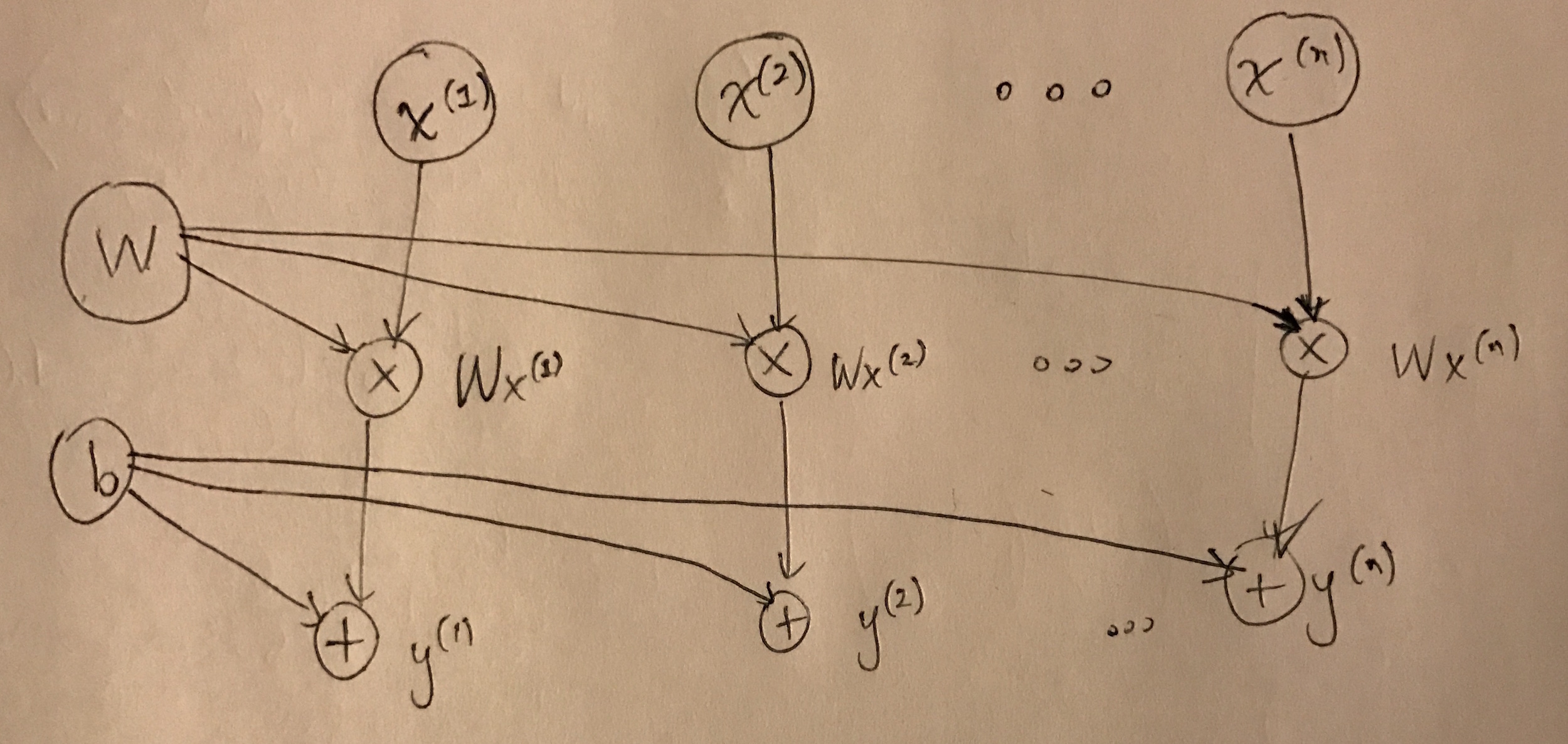
This captures the key property of independence among the samples in \(X\). To compute the local gradients for \(b\), it therefore suffices to compute the local gradients for each of the \(y^{(i)}\) and then add them together. (The rule in computational graphs is to add incoming derivatives, which can be verified by looking at trivial 1-D examples.) The gradient is

See what happened? This immediately reduced to the same case we had earlier, with a \(2\times 2\) Jacobian being multiplied by a \(2\times 1\) upstream derivative. All of the Jacobians turn out to be the identity, meaning that the final derivative \(\frac{\partial L}{\partial b}\) is the sum of the columns of the original upstream derivative matrix \(Y\). As a sanity check, this is a \((2\times 1)\)-dimensional vector, as desired. In numpy, one can do this with something similar to np.sum(Y_grad), though you’ll probably need the axis argument to make sure the sum is across the appropriate dimension.

Affine Layer (Fully Connected), Weight Matrix

Going from biases, which are represented by vectors, to weights, which are represented by matrices, brings some extra difficulty due to that extra dimension.

Let’s focus on the case with one sample \(x^{(1)}\). For the derivative with respect to \(W\), we can ignore \(b\) since the multivariate chain rule states that the expression \(y^{(1)}=Wx^{(1)}+b\) differentiated with respect to \(W\) causes \(b\) to disappear, just like in the scalar case.

The harder part is dealing with the chain rule for the \(Wx^{(1)}\) expression, because we can’t write the expression “\(\frac{\partial}{\partial W} Wx^{(1)}\)”. The function \(Wx^{(1)}\) is a vector, and the variable we’re differentiating here is a matrix. Thus, we’d again need a 3-D like matrix to contain the derivatives.

Fortunately, there’s an easier way with the chain rule. We can still use the rule, except we have to sum over the intermediate components, as specified by the chain rule for higher dimensions; see the Wikipedia article for more details and justification. Our “intermediate component” here is the \(y^{(1)}\) vector, which has two components. We therefore have:

We fortunately see that it simplifies to a simple matrix product! This seems to suggest the following rule: try to simplify any expressions to straightforward Jacobians, gradients, or scalar derivatives, and sum over as needed. Above, splitting the components of \(y^{(1)}\) allowed us to utilize the derivative \(\frac{\partial y_i^{(1)}}{\partial W}\) since \(y_i^{(1)}\) is now a real-valued function, thus enabling straightforward gradient derivations. It also meant the upstream derivative could be analyzed component-by-component, making our lives easier.

A similar case holds for when we have multiple columns \(x^{(i)}\) in \(X\). We would have another sum above, over the columns, but fortunately this can be re-written as matrix multiplication.

Convolutional Layers

How do we compute the convolutional layer gradients? That’s pretty complicated so I’ll leave that as an exercise for the reader. For now.

I just read Keeper of the Olympic Flame: Lake Placid’s Jack Shea vs. Avery Brundage and the Nazi Olympics. This is the story of Jack Shea, a speed-skater from Lake Placid, NY, who won two gold medals in the 1932 Winter Olympics (coincidentally, also in Lake Placid). Shea became a local hometown hero and helped to put Lake Placid on the map.

Then, a few years later, Jack Shea boycotted the 1936 Winter Olympics since they were held in Nazi Germany. Jack Shea believed – rightfully – that any regime that discriminated against Jews to the extent the Nazis did had no right to host such an event. Unfortunately, the man in charge of the decision, Avery Brundage, had the last call and decided to include Americans in the Olympics. (Due to World War II, The Winter Olympics would not be held again until 1948.) The book discusses Shea’s boycott – including the striking letter he wrote to Brundage – and then moves on to the 1980 Winter Olympics, which also was held in Lake Placid.

I enjoyed reading Keeper of the Olympic Flame to learn more about the history of the Winter Olympics and the intersection of athletics and politics.

The book also means a lot to me because Jack Shea was my great-uncle. For me, the pictures and stories within it are riveting. As I read the book, I often wondered about what life must have been like in those days, particularly for my distant relatives and ancestors.

I only met Jack Shea once, at a funeral for his sister (my great-aunt). Jack Shea died in a car accident in 2002 at the age of 91, presumably from a 36-year-old drunk motorist who escaped prosecution. This would be just weeks before his grandson, Jimmy Shea, won a gold meal in skeleton during the 2002 Salt Lake City Winter Olympics. I still remember watching Jimmy win the gold medal and showing everyone his picture of Jack Shea in his helmet. Later, I would personally meet Jimmy and other relatives in a post-Olympics celebration.

I wish I had known Jack Shea better, as he seemed like a high-character individual. I am glad that this book is here to partially make up for that.

One of the advantages of having a four-week winter break between semesters is that, in addition to reading interesting, challenging non-fiction books, I can also catch up on reading academic research papers. For the last few years, I’ve mostly read research papers by downloading them online, and then reading the PDFs on my laptop while taking notes using the Mac Preview app and its highlighting and note-taking features. For me, research papers are challenging to read, so the notes mean I can write stuff in plain English on the PDF.

However, there are a lot of limitations with the Preview app, so I thought I would try something different: how about making a GitHub repository which contains a list of papers that I have read (or plan to read) and where I can write extensive notes. The repository is now active. Here are some papers I’ve read recently, along with a one-paragraph summary for each of them. All of them are “current,” from 2016.

• Stochastic Neural Networks for Hierarchical Reinforcement Learning, arXiv, by Carlos Florensa et al. This paper proposes using Stochastic Neural Networks (SNNs) to learn a variety of low-level skills for a reinforcement learning setting, particularly one which has sparse rewards (i.e. usually getting 0s instead of +1s and -1s). One key assumption is that there is a pre-training environment, where the agent can learn skills before being deployed in “official” scenarios. In this environment, SNNs are used along with an information-theoretic regularizer to ensure that the skills learned are different. For the overall high-level policy, they use a separate (i.e. not jointly optimized) neural network, trained using Trust Region Policy Optimization. The paper benchmarks on a swimming environment, where the agent exhibits different skills in the form of different swimming directions. This wasn’t what I was thinking of when I thought about skills, though, but I guess it is OK for one paper. It would also help if I were more familiar with SNNs.

• #Exploration: A Study of Count-Based Exploration for Deep Reinforcement Learning, arXiv, by Haoran Tang et al. I think by count-based reinforcement learning, we refer to algorithms which explicitly keep track of \(N(s,a)\), state-action visitation counts, and which turn that into an exploration strategy. However, these are only feasible for small, finite MDPs when states will actually be visited more than once. This paper aims to blend count-based reinforcement learning to the high-dimensional setting by cleverly applying a hash function to map states to hash codes, which are then explicitly counted. Ideally, states which are similar to each other should have the same or similar hash codes. The paper reports the surprising fact (both to me and to them!) that such count-based RL, with an appropriate hash code of course, can reach near state of the art performance on complicated domains such as Atari 2600 games and continuous problems in the RLLab library.

• RL^2: Fast Reinforcement Learning via Slow Reinforcement Learning, arXiv, by Rocky Duan et al. The name of this paper, RL^2, comes from “using reinforcement learning to learn a reinforcement learning algorithm,” specifically, by encoding it inside the weights of a Recurrent Neural Network. The hope is that the RNN can help encode some prior knowledge to accelerate the training for reinforcement learning algorithms, hence “fast” reinforcement learning. The slow part is the process of training the RNN weights, but once this is done, the RNN effectively encodes its own reinforcement learning algorithm! Ideally, learning this way will be faster than DQN-based and policy gradient-based algorithms, which are brute-force and require lots of samples. One trouble I had when reading this paper was trying to wrap my head around what it means to “learn a RL algorithm” and I will probably inspect the source code if I want to really understand it. Some intuition that might help: experiments are applied on a distribution of MDPs, i.e., randomly sampling closely-related MDPs, because the high-level learning process must optimize over something, hence it optimizes over the MDP distribution.

• Deep Visual Foresight for Planning Robot Motion, arXiv, by Chelsea Finn et al. This paper takes an important step in letting robots predict the outcome of their own actions, rather than relying on costly human intervention, such as if a human were to collect data and provide feedback. In addition, models that are hand-engineered often fail on real, unstructured, open-world problems, so it makes sense to abstract this all away (i.e. pull humans out of the loop) and learn everything. There are two main contributions of the paper. The first is a deep predictive model of videos which, given a current frame and a sequence of future actions, can predict the future sequence of frames. Naturally, it uses LSTMs. (Note that these “frames” are — at least in this paper — images of a set of objects cluttered together.) The second contribution is a Model Predictive Control algorithm which, when provided raw pixels of the environment and the goal, can determine the sequence of actions that maximizes the probability of the designated pixel(s) moving to the goal position(s). The experiments test nonprehensile motion, or motion which does not rely on grasping but pushing objects, and show that their algorithm can successfully learn to do so with minimal human intervention.

• Value Iteration Networks, NIPS 2016 (Best Paper Award), by Aviv Tamar et al. This introduces the Value Iteration Network, which is a neural network module that learns how to plan by computing an approximate version of value iteration via convolutional neural networks. I think I understand it: the number of actions is the number of channels in a convolutional layer, which themselves represent \(\bar{Q}(s,a)\) values, so by max-pooling over that channel, we get \(\bar{V}(s)\). VINs are differentiable, so by inserting it inside a larger neural network somewhere, it can be trained using end-to-end backpropagation. The motivation for VINs is from an example where they sample MDPs from a distribution of MDPs, specifically for Grid-World scenarios where start/goal states and obstacles are randomly assigned. When training on a fixed Grid-World, a DQN or similar algorithm can learn how to navigate it, but it will be unlikely to generalize on a newly sampled Grid-World. Hence, the agent is not learning how to plan to solve “Grid-World-like” scenarios; it doesn’t understand the goal-directed nature of the problem. More generally, agents need to plan on some model of the domain, rather than a fixed MDP. This is where VINs help, since they enable the entire agent architecture to map from observations to not only actions, but to planning computations. Another contribution of their paper is the idea of using another MDP, which they denote as \(\bar{M}\) along with the subsequent \(\bar{s}, \bar{\pi}\), etc., and then utilizing the solution to that for the original MDP \(M\).

• Principled Option Learning in Markov Decision Processes, EWRL 2016, by Roy Fox et al. This paper is about hierarchical reinforcement learning, where the “sub-policies” at the base of the hierarchy are called “options”, and the higher-level policy is allowed to pick and execute them. This paper assumes a prior policy on an agent, and then uses information theory to develop options. For instance, in a two room domain, if we constrain the number of options to two, then one option should automatically learn to go from left to right, and another should go from right to left. The hardest part about understanding this paper is probably that there is no clear algorithm that connects it with the overall MDP environment. There’s an algorithm there that describes how to learn the options, but I’m still not sure how it works from start-to-finish in a clean MDP.

• Taming the Noise in Reinforcement Learning via Soft Updates, UAI 2016, by Roy Fox et al. This paper introduces the G-learning algorithm for reinforcement learning, which I’ve correctly implemented (I hope) in my personal reinforcement learning GitHub repository. The central motivation is that the popular Q-learning algorithm learns biased estimates of the state-action values due to taking the “max” operator (or “min” in the case of costs). Therefore, it makes sense to use “soft updates” where, instead of taking the single best “successor action” as in the standard Q-learning temporal difference update, we use all of the actions, weighted according to probability. This is, I believe, implemented by imposing a prior policy on the agent, and then formulating an appropriate cost function, and then deriving a \(\pi(a'|s')\) which enforces the “softness.” The G-learning algorithm relies on a tuning parameter which at the start of training values the prior more, and then as time goes on, G-learning gradually shifts to a more deterministic policy. The G-learning update is similar to the Q-learning update, except it uses information-theory to mitigate the effect of bias. I haven’t been able to do the entire derivation.

Aside from these papers being Artificial Intelligence-related, one aspect that seems to be common to these papers is the need for either hierarchical learning or increased abstraction. The former can probably be considered a subset of the latter since we “abstract away” lower-level policies in lieu of focusing on the higher-level policy. We can also abstract away the process of choosing MDPs or a pipeline and just learn them (e.g., the Deep Visual Foresight and the RL^2 papers). That might be something useful to keep in mind when doing research in this day and age.

[Warning: long read]

Last year, I wrote a normal-length blog post about my three favorite books that I read that year. For 2016, I thought I would do something a little different: why not list all the books I read this year? That way, I won’t forget what I read, and if anyone complains to me saying “why do young adults nowadays spending time on social media instead of reading books?”, I can simply refer them to my blog. Genius!

I have done precisely that in this lengthy post, which I’ve been updating throughout the year by writing summaries of books as soon as I’ve finished them. I read 38 books this year. (Textbooks, magazines, newspapers, and research papers don’t count.) The summaries here are only for the non-fiction books that I read this year. I read three easy fiction books in January to get me warmed up,¹ so the summaries here are for the other 35 books. Here’s a rough set of categories:

1. Medicine and Surgery (4 books)
2. Work Habits and Technology (4 books)
3. History and Foreign Affairs (5 books)
4. Religion (5 books)
5. Science (4 books)
6. NSA and CIA (3 books)
7. Biographies and Memoirs (3 books)
8. Miscellaneous (7 books)

Books I especially liked are indicated with double asterisks by the title, ** like this **. For the full set of these “reading list” posts, see this page.

Group 1: Medicine and Surgery

I read all of Atul Gawande’s four books. Gawande is a famous surgeon who also gave the 2012 commencement speech for my alma matter. I think he’s an excellent surgeon-writer. His books contain a healthy amount of technical detail on surgery and medicine without going overboard to discourage the lay reader like myself. They not only give me a glimpse into what it must be like to work in medicine, but also make me appreciate my relatively good physical health. Some of the stories Gawande describes about his patients are absolutely shuddering.

Here are my thoughts on his books:

• Complications: A Surgeon’s Notes on an Imperfect Science, Gawande’s first book and a finalist for the National Book Award, discusses the various complications and uncertainty that arise in surgery and medicine. It is divided into three parts: fallibility, mystery, and uncertainty. What happens when doctors make mistakes? And how do people feel about an inexperienced surgeon working on them? (After all, everyone has to start somewhere!) What about when there are cases that simply elude everyone? How about pure judgment calls? Each of the fourteen chapters covers a certain theme, and consists of several related stories. It’s a nice portrayal of how medicine faces some of the inherent difficulties in its field.

• Better: A Surgeon’s Notes on Performance. Gawande explores different ways to get “better” at surgery and medicine. Like his last book, this one is a collection of loosely-related stories. In general, Gawande doesn’t directly propose solutions to various issues, but rather, he provides examples of how certain people at the top of their field (e.g., those treating cystic fibrosis) carry out their work, in comparison to “ordinary” people. There are also some interesting but awkward topics: how should physicians treat the handling of patient genitals, and how should doctors discuss their “bell curve” of performance and the possibility that they may be at the lower tail? While the book is a nice collection of stories, the selection and ordering of topics might seem somewhat haphazard. Still, I felt that – like other books – it gave me a glimpse into what it is like to be a surgeon.

• ** The Checklist Manifesto: How to Get Things Right ** is an enlightening book about the power of checklists. Drawing from a variety of fields, including airfare, construction, and (obviously) surgery, Gawande shows how checklists have increased the safety and efficiency of those tasks that most of us take for granted. Yes, he acknowledges that checklists are stupidly simple. But here’s the remarkable thing: why didn’t anyone else write about this earlier? And why, as Gawande points out, do people resist utilizing something enormously beneficial with virtually no extra cost? Consequently, I’m now thinking about where checklists might be applied to my own life. One qualm I had with this book, however, is that it seems to put a ton of statistics in terms of percentage points only (e.g., 22 percent said this …) whereas we need the raw number to understand the significance (e.g., 22 percent of 10000 people surveyed …). This book is on the short end (fewer than 200 pages) so it wouldn’t hurt to have a little more data and facts.

• ** Being Mortal: Medicine and What Matters in the End **. What is the role of doctors when treating patients who are near the end of their lives? Surgery and medicine often restrict their focus to “fixing stuff:” if a patient has a problem, then doctors should undergo the procedure that will prolong patient’s lives the most. But what if that leads to the patient going directly into a nursing home? What if the patient and his/her family are banking on being the one-percent of people who end up significantly better off after a specific procedure? Most examples of patient stories in Being Mortal concern cancer, a notoriously difficult disease to treat, and people are not always willing to undergo brutal surgery and chemotherapy. I should point out that this is not a book on assisted suicide; the book only dedicates about four pages to that topic, towards the very end. Rather, this book is about assisted living; how can we balance patient’s desires while considering their safety and their relatives’ (sometimes conflicting) desires? I liked this book a little more than I liked The Checklist Manifesto, and it made me think about what I would want to happen to my older relatives. And, of course, myself, but hopefully I won’t have to worry about that for a long time.

Group 2: Work Habits and Technology

In this group, I have two books by Georgetown computer science professor Cal Newport. I first became aware of Professor Newport’s blog back in high school when I Google-d “how to get good grades in college.” That search led me to a College Confidential thread which subsequently linked to his blog.

Professor Newport is a voracious reader (which I hope to be as well), so he recommends and discusses a number of books on his blog. I chose to read two of them.

• So Good They Can’t Ignore You: Why Skills Trump Passion in the Quest for Work You Love. Here, Newport argues that the often-cited “follow your passion!” suggestion is actually terrible, and people are better suited at developing skills that will allow them to eventually figure out their dream jobs. In short: don’t quit your job now with the fantasy that you’ll enjoy this new thing you’re starting out next week – you’ll end up worse than you were when you started. It is true that I sometimes feel like I may not be in an ideal job for me, but then I think things over, and realize that the current PhD program I’m in is clearly training me for a lot of jobs. Even if being a professor isn’t in the cards for me, I’m still learning a lot about programming, about advanced computer science, about teaching, about making connections, etc. Thus, this book made me feel happy that I am spending my twenties in an intellectually stimulating environment where my main responsibility is to learn new things and blog.

• ** Deep Work: Rules for Focused Success in a Distracted World **. This is Professor Newport’s most recent book and arguably his best, which became a Wall Street Journal 2016 business bestseller. His hypothesis here – which was obvious to me from the start – is that deep work, which is a state in which one is able to focus very heavily on a topic, churning out lots of work in a short amount of time, is becoming rarer at a time when it’s becoming more valuable. The former is due to distractions from smart phones and social media, and the latter is because the knowledge economy means people can pay the best workers remotely rather than hire locally for less-skilled people. When I was reading this book to myself, I kept thinking: come on, why on earth am I not engaging in deep work? There’s a lot of advice here, and there’s no way I can integrate them all, but I’ve been able to take a few steps (e.g., as my Facebook “friends” can attest, I don’t check Facebook frequently, and I don’t have Twitter, Instragram, SnapChat, or whatever is popular nowadays, and I check my smart phone a lot less than most people). I agree with a lot of what Newport says here; it seems like so much common sense. I have to add, it’s also funny that this book got published at a time when a related Deep phenomenon called Deep Learning is hot in AI, but that’s a story for another day.

• You Are Not a Gadget: A Manifesto, recommended by Professor Newport, is a 2010 book written by Jaron Lanier, one of the pioneers of virtual reality technology. Lanier worries that our early technological achievements have locked us in into suboptimal paths. In addition, he argues that many areas of technology are dehumanizing and favor the crowd or algorithm over individual human voices. To me, while it’s true that Wikipedia may be dehumanizing in some sense, things were arguably much worse pre-Wikipedia from a “dehumanizing perspective” (NOT a technological perspective). To take one example, as Robert Gordon describes in his fantastic book The Rise and Fall of American Growth², human life before the “great inventions” from 1870-1970 was extremely isolating, particularly for rural families and farmers (and this continued to be the case in this era for many areas of the U.S., particularly in the Civil War-ravaged south). If a family is isolated from the rest of the world, that seems pretty dehumanizing to me. Overall, as you might tell, I have some mixed feelings about this book and do not revere it as much as Professor Newport, but it certainly brings up thought-provoking points.

• Throwing Rocks at the Google Bus: How Growth Became the Enemy of Prosperity is a 2016 book by Douglas Rushkoff, which I became aware of after reading (guess what?) one of Cal Newport’s blog posts. The author of this book is an American media theorist (what’s that?) and this book provocatively argues that our economic “operating system” of capitalism is not the best for today’s world. The latest technology boom creates value not with real things, but with human data. In addition, it encourages start-ups to create value for shareholders instead of “the people”, and to sell immediately instead of generating revenue. Rushkoff heavily criticizes our obsession³ with economic growth mindset, arguing that further growth is limited and doesn’t actually provide much value beyond the top 1 percent. Instead, Rushkoff argues that we need to stop this growth mindset and ensure that business is designed to be peer-to-peer (as in, more like eBay, not Amazon!) and to re-introduce humans into the equation. This is not meant to be income redistribution; it’s meant to ensure that business can work more towards an equal distribution of wealth. He heavily criticizes Amazon, Uber, WalMart, and other companies whose goal is to destroy competition rather than to create value. From reading this book, I definitely became concerned about whether I’m exacerbating the issue by supporting Silicon Valley ideals (I use Uber, and Amazon …) and am ignoring the realities of how most people live. This book is something that I will try to remember and to extract policy solutions from. I get the feeling that many pro-business Republicans may be skeptical of his proposals. Even though they’re technically centrist, it may sound more like liberal/socialism policies, but I would urge readers to consider this book.

Group 3: History and Foreign Affairs

Another way for me to describe this category would be “Thomas Friedman and Michael Mandelbaum books” since all of the books in this category are written by them (in fact, one is co-authored by them!). For better or worse, most readers probably know Thomas Friedman from his columns at the New York Times. Michael Mandelbaum is professor emeritus at Johns Hopkins University, specializing in international affairs. I enjoyed these books.

• ** From Beirut to Jerusalem ** is a fascinating book about Thomas Friedman’s journey through the Middle East from 1979 to 1989, when he worked as a reporter and got to witness firsthand the people of Lebanon and Israel. The first half the book discuss his experience living in Beirut (in Lebanon). The second half of the book focuses on his life in Jerusalem, a religiously important city for Christians, Jews, and Muslims. The city was (and still is) hotly contested by Israelis and Palestinians. Throughout the book, Friedman discusses some history about how the Middle Eastern countries developed and why they are in constant conflict, but he also takes his reporting ability into account by describing detailed conversations and events he has witnessed. His extensive dialogue, his seemingly random thoughts about life, and his colorful analogies serve as intuition for what it must be like to live there. (In other words, I view this book as a textbook in how it teaches the reader about the Middle East, but the “teaching” is not through textbook-style language.) I do not know much about the Middle East, and even after reading this book, I still feel that way. But I sure think this book gave me a jump start in forming a baseline set of knowledge that I can draw upon when reading more books about the Middle East (and yes, there will be more!). The book, though old with its 1989 publication date, is still relevant today as the Israeli-Palestinian conflict proceeds without any end in sight. The focus on the Middle East nowadays has probably shifted from Lebanon to countries such as Saudi Arabia and Iran (due to terrorism and oil) and Syria (due to the refugee crisis and Assad) but Israel is still a major player for US diplomacy and foreign policy, and reading this book will be helpful in the process of better understanding the parties involved in the Middle East.

• ** The World is Flat: A Brief History of the Twenty-First Century ** is a long book by Thomas Friedman. I read the third edition, published in 2007; the first two were published in 2005 and 2006. The metaphor “the world is flat” refers to the forces of globalization that have connected various people and countries together, and which empower the individual, particularly the Internet and how it allows people to have their own voices with blogs. (Contrast this, by the way, with Jaron Lanier’s book above, who argues that the Internet has been a chief cause of de-empowering the individual.) To his credit, Friedman emphasizes that globalization has tradeoffs. A frequent theme is the offshoring of work; companies can improve profits by utilizing cheaper labor in China and India, which benefits American consumers but makes life harder on those former American workers. Globalization has impacts on politics, of course, because it heightens income inequality. Friedman is pro-free trade, but understands that we have to provide the education and opportunity for people to flourish in this world. Right now, he argues America is not doing anywhere near as well as it should be doing — a quiet education crisis. This book is definitely a good history lesson for me, and it completely changed my perspective on how the world works.

• The Frugal Superpower: America’s Global Leadership in a Cash-Strapped Era is a short book written in 2010 by Michael Mandelbaum. Its central argument is that in the twentieth century, America effectively served as the world’s government and was able to intervene in other countries because it had the money to do so. But after the 2008 financial crisis, a shift emerged in U.S. policy: no longer can we lavishly spend money and intervene almost at will. Mandelbaum, while recognizing that it is not optimal to have financial crises, hopes that we can be more circumspect (hence, a “frugal” superpower). We will, however, have problems because of entitlement spending, which naturally implies spending less on military action. Demography is also working against us, but the saving grace is that the three areas of contention (Russia, China, and the Middle East) all have their own problems. For example, China has even more of a demographic problem due to their former one-child policy. Mandelbaum concludes that one way we can restore the world order is by taxing gasoline, so (a) we reduce profits of Middle Eastern countries (and indirectly, I might add, radical Islam), (b) provide more money to the federal government for entitlements, and (c) we encourage renewable and cleaner energy, thus helping to combat climate change. This book, with the exception of the suggestion that we tax gasoline, is largely subsumed by Mandelbaum’s later book, Mission Failure.

• ** That Used to Be Us: How America Fell Behind in the World It Invented and How We Can Come Back **, co-authored by columnist Thomas Friedman and foreign policy professor Michael Mandelbaum, is a book arguing that America is failing to meet the four major challenges of today’s world: globalization, the IT revolution, chronic deficits, and increasing energy consumption. The authors look at America’s history and see many examples of how we have been able to overcome similar challenges. Unfortunately, they worry, “that used to be us.” Today, with our political gridlock, lack of education funding, and competition worldwide from Asia, especially from China (who they almost view as being the most powerful country in the 21st century), it is uncertain whether we will be able to resolve these problems before the market or Mother Nature brutally forces changes down our throats. One of their main solutions? A third-party presidential candidate on the “radical center” who, while not necessarily winning the election, would sufficiently influence the two parties to focus on the “radical center” issues, as H. Ross Perot did in the 1992 election about balancing the deficit. I really liked this book, and I agree with Bill Gates’ assessment that the one word review of this book is: “fascinating.” Not everyone would like this, however: the Wall Street Journal published a negative review, taking a traditionally Conservative stance by criticizing the authors for proposing more government as the solution to fixing America. But then I would like to ask them: what is their proposal to combat climate change?

• ** Mission Failure: America and the World in the Post-Cold War Era ** is Michael Mandelbaum’s fifteenth and most recent book, published in 2016 and dubbed by Thomas Friedman as “a book that Barack Obama and Donald Trump would both enjoy”. The focus is on the period starting from 1991 — the Cold War’s end — to 2015. In this period, spanning four American presidents (George H.W. Bush through Barack Obama), Mandelbaum argues that we spent this time, intentionally and unintentionally, engaging in “regime change” in other countries. The goal? To convert them to Western-style countries supporting peace, democracies, and free markets. Those three features are the foundations of Mandelbaum’s 2002 book The Ideas that Conquered the World, one of my favorite books and one which I blogged about last year. As examples, the Clinton administration engaged in substantial humanitarian intervention in countries that had little significance to the U.S., such as Haiti, Somalia, Bosnia, and Kosovo. The Bush 43 administration also engaged in nation building in Iraq and Afghanistan, though this was not the original goal as in both cases, it started from war. In addition, for many years we have tried to convert Russia, China, and other middle eastern countries (especially Iran and the Palestines) to be more like ourselves. But these missions all failed. Why? Probably the biggest reason is culture; in many countries, there is already so much sectarian violence that unity based on abstract concepts like the “rule of law” is not possible. In other cases, there is American resentment, as in Russia due to NATO expansion. I found the history behind all this to be fascinating. Of course, I am also concerned. After all, this “era” of American foreign policy abruptly ended by 2015, because Russia and China have now become powerful enough to upset the stability of global order.

Group 4: Religion

Here are some religion-related books. Specifically, these are from the non-religious or atheist perspective, which one might be able to tell given Sam Harris’ frequent appearance here. Don’t worry, I’m going to explore with more pro-religion books next year, and my parents have several book candidates which I can read.

• Moral Minority: Our Skeptical Founding Fathers, by Brooke Allen, argues that the six men who she considers to be the founding fathers of America: Benjamin Franklin, George Washington, Thomas Jefferson, John Adams, James Madison, and Alexander Hamilton, were not devout Christians as many claim, but instead highly skeptical men influenced not by religion, but by John Locke and Enlightenment thoughts. By doing so, Allen further claims that due to the efforts of these men, the United States was not founded on Christian principles. (To me, I find it odd that we’re often considered a “Christian nation” when the First Amendment explicitly allows for Freedom of Religion — and don’t get me started on “Judeo-Christian”.) The book has one chapter for each of these men, and uses their actual writing to claim that they were skeptical of religion and preferred to keep it out of politics. I agree with the main ideas of Moral Minority, but rather surprisingly (to me), I didn’t enjoy the book. In part this is due to the writing style; it’s a lot harder to understand 18th-century writing than modern writing. I also think the book discusses a lot of facts but doesn’t clearly unify or connect them together.

• ** The End of Faith: Religion, Terror, and the Future of Reason ** is Sam Harris’s first book, written in 2004 while he was still a Ph.D. student⁴ in neuroscience. Its impact was remarkable: it propelled him to fame and played a critical role in forming the New Atheist movement. Harris began writing on September 12, 2001, when the ashes of 9/11 were well present, and the essay he produced in those weeks of collective grief became the basis for this book. This book is similar to Richard Dawkins’ The God Delusion (blogged about here) in many ways, in that it is highly critical of religion, though to be clear: this is about criticism of sticking to any particular dogma, not necessarily religion. In fact, Harris argues near the end of the book (and this is something I did not know from reading Dawkins’ book) that Buddhism as a religion is far more an empirical science than Christianity, Islam, and Judaism. While Dawkins focuses more on the Bible and Koran and argues for evolution instead of creationism and intelligent design, Harris here takes more of a “mind and consciousness” route, which suits his philosophy and neuroscience academic background. One particular aspect about the book is that he is especially critical of Islam, which should not strike readers as surprising, since he argues that religion must be the driving force behind suicide bombing, etc. While I recognize that there are many controversial aspects of Sam Harris and his books, I personally liked this book a lot and view Harris highly. I agree with him that any discussion of religion must begin with the thousands of people who lost their lives on September 11, 2001.

• The Moral Landscape: How Science can Determine Human Values, a 2010 book by Sam Harris, argues that people are mistaken about moral values. He urges us to think about improving “well-being” as being equivalent to a peak in a hypothetical, non-convex (to use a term from math) “moral landscape”. This book, while not as anti-religion as his others, dismisses religion as something that causes people to be too rigid to change, and creates friction over “distractions” (social issues such as gay marriage) when we really should be focusing on the threat of terrorism, climate change, and – of course – how to best advance the collective well-being of humans. In my opinion, I was reminded of the Moral Minority book by Brooke Allen – I can find myself agreeing with the general idea, but I felt like the argument is somewhat haphazard and it took me some re-reads of certain paragraphs to get his ideas. Honestly, to me his biggest claims come from arguing that there are other sciences that are vague and have subjective answers (e.g., health and economics) so morality should not be subject to a double standard. Note that he has an interesting discussion of this book on his blog where he challenged readers to refute his thesis.

• Waking Up: A Guide to Spirituality Without Religion is a 2014 book, also by Sam Harris, that delves into rather unusual terrain for atheists: spirituality. I read this book for two reasons: one is that I know Sam Harris’ work and admire it very much, and the other is that I have been looking for spirituality or “meditation”-related stuff for a while to help decrease stress. This book, however, is less a “guide on spirituality” that its title suggests, and more about a discussion of the mind, the self, and consciousness. That I find really illuminating, albeit considerably difficult to understand. I felt lost many times in the book and had to reread certain sections, trying to gather every ounce of understanding I could. As an atheist, I acknowledge that there are very real benefits of spirituality and meditation, and that these can be utilized without religion. I want to pursue some of these tactics, but preferably those that don’t involve drugs, as Harris talks about near the end of the book. Ultimately, I was disappointed not because it is a bad book, but because I was expecting to get something different out of it.

• Islam and the Future of Tolerance: A Dialogue, yet another book by Sam Harris (co-authored with Maajid Nawaz in 2015) is a conversation between the two men, who come from two vastly different backgrounds. Sam Harris is a well-known atheist, and I frequently read his blog and books (as highly suggested by this blog post!). Nawaz has a remarkable personal story; he was born in England, but became radicalized, but then escaped to become a liberal Muslim activist. Harris and Nawaz have a dialogue about Islam and the prospects of reforming the faith. Nawaz urges us to have plurality, which will lead towards secularism, while Harris argues that we need to start viewing Islam directly as the problem because the accurate reading of scripture indicates that it is among the more evil of religions. I was impressed that two men who no doubt have disagreements can have an honest dialogue, even if the difference isn’t that great (Nawaz doesn’t strike me as a super-religious person). But we need a starting point if we are going to counter radical Islam. I wrote a blog post about it earlier this year in the wake of the Orlando massacre.

Group 5: Science

Needless to say, given my “job” as a computer science graduate student, I have an interest in excellent (popular) science books. Here are four of them. The first three are physics/earth/biology-related with nontrivial overlap in their topics. The last one one is a machine learning book.

• What Evolution Is, by famed biologist Ernst Mayr, is a 2001 book about evolution aimed at the educated non-biologist. It is almost like a textbook, but simpler (the book itself is barely 300 pages). Mayr argues that evidence is not merely a theory, but a fact, based on the evidence of evolution from the fossil record. Mayr takes pains to show that this did not come out of a creationist-like reasoning of saying “this is a fact”; rather, the current theory of evolution based on natural selection had several competing theories when biology was in the early stages as a subject. Gradually, as the evidence accumulated, biologists more or less came to a consensus on the current “theory”. This is an extraordinary example of science in action. Ultimately, I don’t quite go as far as Jared Diamond (author of Guns, Germs, and Steel), who says that this book is the “second-greatest thing” that could ever happen, with the first being if Darwin himself (the most famous biologist of all time) came and wrote a book about this. But the book is educational since it’s written like a pseudo-textbook. It’s somewhat dry to read but with enough effort, you can understand the main ideas.

• The Sixth Extinction: An Unnatural History, by Elizabeth Kolbert⁵, is an engaging fast-paced book arguing that we are in the middle of the next mass extinction — the sixth of the earth’s history. (The fifth, of course, was the one that wiped out the dinosaurs, a key topic of Lisa Randall’s book, which I’ll describe next!) The Sixth Extinction consists of a series of short stories documenting Kolbert’s adventures across the world, where she meets lots of people and explores the outdoors. Some conditions are dangerous, and others are more amusing, as when she recounts seeing frogs having sex. But where there is humor is also sadness, because the story of extinction is not pleasant. Kolbert describes how biologists have failed to find once-abundant frogs, how zoologists have had to deal with the reality of trying to force the two remaining fertile members of a species to create offspring, and how the effects of ocean acidification and human-accelerated climate change will accelerate extinction. This book, however, is not about global warming, as that subject plays only a minor role here. Even discounting global warming, there is irrefutable evidence that humans have directly caused the extinction of other species, whether it is through construction projects, deforestation, transporting pests across the world, and other actions. After reading this book, I continue to remain concerned about the future of the world and the fate of our species.

• ** Dark Matter and the Dinosaurs: The Astounding Interconnectedness of the Universe **, by famed cosmologist and physicist Lisa Randall, is an exciting book weaving together astronomy, particle physics, earth science, and biology, to answer a profoundly interesting question: what caused the dinosaurs to die? No, I don’t mean about the meteor that hit earth. We know all that, and Randall briefly describes the interesting history of how scientists arrived at that conclusion. Randall’s book is instead about what caused the meteor to hit the earth. That’s a much more challenging question, and for someone like me without formal astronomy education, I have no idea how people can answer that kind of question considering the immense complexity and size of the universe. Fortunately, Randall explains the astronomy and particle physics basics for understanding some of this material. She proposes the new, very preliminary hypothesis that a disc of dark matter caused the meteor to hit the earth. The dark disc in the solar system causes the sun and planets to move up and down in unison periodically, and due to certain gravitational influences, when passing the center of the disc, causes one of the meteors (perhaps in the Oort cloud, something cool I learned) to dislodge from its orbit and sends it to earth. After reading Dark Matter and the Dinosaurs, I can no longer view the universe the same way. It is an exciting world we live in, and though I will not be part of the physics/cosmology research that explores Randall’s hypothesis, I eagerly await what they find and hope that Randall will write another book in five years describing her research progress.

• ** The Master Algorithm: How the Quest for the Ultimate Learning Machine will Remake Our World ** by Pedro Domingos is one of the few popular science books on machine learning, so naturally, I had to read it. It describes the history of machine learning as five tribes: symbolists, connectionists, analogists, Bayesians, and evolutionaries. This is what I wanted to know, so I’m happy he included this in his book. Near the end of the book, I felt like Domingos went a bit overboard with storytelling, but it’s probably better than the alternative of having more math. Certainly I would prefer more math, but most readers probably don’t want that, and we need ways to teach machine learning to a broad audience without much math. I have covered my thoughts on this book more extensively in this blog post. It’s an interesting book, to say the least, and I wish there were more books about this general area.

Group 6: NSA and CIA

I maintain an interest in the NSA and the CIA. I chose three related books to read and I liked all of them. This is despite how two books ostensibly appear to be on the opposite side of a contentious political issue (NSA collection of bulk metadata). The third is an espionage thriller … which happens to be true.

• ** No Place to Hide: Edward Snowden, the NSA, and the U.S. Surveillance State **, is a 2014 book by journalist Glenn Greenwald. He was one of the people who Edward Snowden first contacted about the release of classified NSA phone metadata collection documents. The first part of the book is quite riveting, since it describes how Snowden first attempted to contact Greenwald (via PGP email, but that never happened) and how Greenwald decided to go to Hong Kong to meet Snowden. Greenwald next takes Snowden’s side regarding the NSA’s actions and argues that Snowden is right about what the NSA does (as in, Snowden’s famous “I, sitting at my desk, could wiretap you […] if I had a personal email” phrase). Greenwald displays a number of leaked documents to support his arguments. Next, Greenwald argues that government spying is bad. Privacy is a fundamental human right, and government spying encourages conformity and suppresses valid dissent. One passage that particularly struck me was when Greenwald said that the alternative to mass surveillance is not no surveillance, but targeted surveillance. This is a lesson that might be useful to many policymakers today.

• ** Playing to the Edge: American Intelligence in the Age of Terror **, a 2016 book by Michael V. Hayden, the only person to be the director of both the National Security Agency and CIA. It is meant to be “an unapologetic insider’s perspective” on the organizations in a time of terror, but also a time of criticism from the general public, who do not understand the intricacies of what these agencies do and what they are legally bound to do. Mr. Hayden frequently mentions that the NSA and CIA are unfairly asked to do more when the public feels unsafe, but then they’re asked to do less when the public feels safe. Mr. Hayden discussed his time talking to Congress, the POTUS (usually Bush 43, but he was also Obama’s CIA chief for three weeks), and other politicians, in an attempt to keep them as informed as possible, but that nonetheless did not seem to satisfy many Libertarians and others who oppose aspects of the work of the NSA and CIA. I found this book fascinating mostly for the insider’s perspective on what it’s like to manage such critical government organizations, and the careful considerations of these organizations when pursuing sensitive strategies (e.g., the metadata collection). I wish that there were other secrets he could have discussed, but I understand if this is not possible. One possible weakness is that it’s more of a biography/memoir with loosely related chapters, and doesn’t do enough (in my opinion, if it was the goal) to directly counter people like Glenn Greenwald⁶ and others who oppose NSA bulk collection of phone records.

• ** The Billion-Dollar Spy: A True Story of Cold War Espionage and Betrayal ** is a 2015 book written by David Hoffman. The book’s summary in its cover flaps describes it as “a brilliant feat of reporting which unfolds like an espionage thriller”, and I think this is a valid description. I thoroughly enjoyed the book’s details on Cold War espionage activities performed by the US and the Soviet Union (and this is something getting more attention nowadays due to Obama’s much-needed sanctions on Russia). It emphasizes how U.S. spies had to carefully communicate with Soviet engineer-turned-spy Adolf Tolkachev deep into the heart of Moscow … and several blocks away from the feared KGB. Fortunately, they were able to do that for several years, continually communicating with Tolkachev who handed over tens of thousands of secret documents. The air force said the material was worth “roughly in the billions of dollars range”. Wow. But then, in 1985, the operation ended due to a shocking betrayal. There are several downsides to this book. The first is that the “betrayal” is obvious once the appropriate character is introduced, and the second is that it includes some nice pictures of the characters and setting, but the pictures should be at the end of the book (not the middle!) because it gives away the ending. The first is a limitation of the story, though, and the alternative would have been to expand the book to be longer and introduce more characters early. I still greatly enjoyed this book, a riveting and poignant tale of Tolkachev.

Group 7: Biographies and Memoirs

Here are some biographies and/or memoirs, with quite different themes. Actually, Michael Hayden’s book (from the previous group) would also qualify as a memoir.

• What I Talk About When I Talk About Running is the first book by Haruki Murakami that I’ve read. Murakami is mostly known as a prominent fiction writer, both in Japan and abroad, but I decided to read this book since I was in the middle of a personal “Running Renaissance” (e.g., see this blog post about running in the Berkeley Marina) and wanted to see his take. This book is a short memoir about the notes (most from 2005/2006) Murakami compiled while training for the New York marathon. Along the way, we learn that Murakami ran a bar (in Japan) until his thirties, but then started writing and struck gold there. He then started running to help him physically manage the strain of writing novels. Regarding his running, Murakami describes his experience training and running in marathons once a year. He’s even run an ultramarathon in Lake Saroma, which is 62 miles long. This book is probably an accurate survey of what Murakami thinks, though I think it suffers a lot from cliches: hard work can beat talent!, most people need to work hard!, and so forth. It’s a short book so even if one doesn’t like the concepts, reading it from start to finish does not take much time.

• Between the World and Me by Ta-Nehisi Coates, an author (and MacArthur Fellow) who I was previously aware of due to his 2014 The Case for Reparations article. This book won the 2015 National Book Award, so I was looking forward to reading it. The best way to describe this book is as a cross between a long letter and a poem, and Coates addresses it to his son. He argues that, as blacks, they will have to be extra careful about their bodies. He says that there is a lot of concern in a world where we’ve recently seen a lot of police officers shooting black men and boys. (And, tragically, the manuscript for this book must have finished before the Charleston shootings, which certainly would have made it in otherwise.) One term he uses a lot is “The Dream”, but paradoxically, it doesn’t actually seem to refer to a dream for blacks (as in, Martin Luther King Jr.’s kind of dream) but that of whites who are attempting to define themselves. In terms of my opinion, it’s true that this book helps me to understand the perspective of being black, and obviously made me appreciate not being black⁷. I think Coates could have focused more on the shooting cases where the officers were clearly guilty or had video evidence suggesting that, because in some cases it is justified for police officers to retaliate. Whether they did or not in those well-known cases, is not my place to answer, and could be a source of fair criticism for this book. As for the title, I think it was designed to represent how there is a “real” world, one for whites, and “his world” of blacks.

• Sisters in Law: How Sandra Day O’Connor and Ruth Bader Ginsburg Went to the Supreme Court and Changed the World is a 2015 dual biography by lawyer Linda Hirshman. She describes an overview of the Justices’ lives, starting from childhood, then to their difficulty establishing legal careers, and of course, to their time as Supreme Court justices. The book is educational for those who want to know about the politics and intricacies of the Supreme Court. I certainly count as one of those, so this book was a nice match for me: it was just technical and sophisticated enough that I could follow it (along with some Wikipedia checks to, for instance, understand what it really means to clerk for a judge or to be on the United States Court of Appeals). I also learned a lot about how the court works, about how justices have to strategically frame their arguments to get a majority, and why it matters who writes the opinions. The book talks about Ginsburg’s rise, then O’Connor’s rise, then about them together later. Towards the end of the book, Hirshman starts intervening with her personal opinions, as well as her attacks on Justice Anthony Kennedy. Hirshman doesn’t shy about inserting her liberal beliefs so this may discomfort diehard conservatives (but not moderate conservatives, ironically those like O’Connor), and I wonder if she would have done something differently had she waited until Kennedy wrote the majority opinion which legalized same sex marriage. I enjoyed knowing more of the relationships between the Supreme Court justices and how they work, and would like to see more of that if the book were to be extended. Also see the book’s review on the “nonpartisan” SCOTUS blog, which I mostly agree with.

Group 8: Miscellaneous

These are some miscellaneous books, which don’t seem to fit in the above groups. I’ve arranged them by publication date.

• The Swerve: How the World Became Modern is a 2011 book by Harvard professor Stephen Greenblatt that won the 2011 National Book Award and the 2012 Pulitzer Prize (geez …). It’s the story of how Poggio Bracciolini, an Italian scholar and book-hunter in the 14th and 15th century, was able to track down Lucretius’ On the Nature of Things, a dramatic, profound essay that had been lost for well over a thousand years, and (incredibly) describes things that we take for granted today, especially the atomic nature of the world. The book chronicles Poggio’s journey to get the book and navigates through his life as a papal secretary and, clearly, the trip that led him to reach the long-lost manuscript. Note that this book is technically non-fiction, but given that this all happened in the 1400s, I think some of its content is bound to be the result of artistic license. Greenblatt argues that this essay “revolutionized our understanding of the world we live in today.” I thought this book was interesting, though I probably wouldn’t be on record as saying it was as great as other books I’ve read, such as Guns, Germs, & Steel. One thing that might not suit certain readers is the anti-religious stance of On the Nature of Things, which argues that there is no afterlife, so it subscribes to the Epicurean philosophy that life should be fulfilled for enjoyment first. For instance, see Jim Hinch’s criticism of the book.

• David and Goliath: Underdogs, Misfits, and the Art of Battling Giants is another book (from 2013) by the famous author Malcolm Gladwell, who I regard as one of the finest authors for explaining how the world works. I thoroughly enjoyed reading The Tipping Point, Blink, and Outliers in high school. This book is about taking a new perspective of underdogs versus the favorites. Why are we surprised when the underdogs win? What if we should expect underdogs to win? Gladwell discusses how people with disabilities or traumatic experiences, while generally worse off than others, have a chance of overcoming and being stronger than ever. For instance, he cites David Boies, a dyslexic lawyer who countered his disability with the ability to listen far better, and he is one of the top tax lawyers in the country. He also raises the interesting point as to whether it is better to be a big fish in a small pond or a little fish in a large pond. The first two parts are my favorite; the third part is a bit drier and mostly discusses how people who are in power have to consider carefully what happens to those under them (e.g., police officers versus civilians, the United States versus (North) Vietnam, etc.). Overall, the book, especially the first two parts to me, is thought-provoking and I agree with a lot of what Gladwell says. I do, however, have to emphasize a criticism of the book that I’ve seen declared elsewhere: when students who are at schools of vastly different prestige study the “same” subject, they are not studying the same concepts, looking at the same notes, etc. I can say this with confidence after studying the material from the artificial intelligence and machine learning courses at Williams and at Berkeley⁸. The Williams courses are noticeably easier and cover less material than the Berkeley counterparts. And Williams is a very strong school in its own right! The gap is therefore wider for other pairs of schools.

• Kill Anything That Moves: The Real American War in Vietnam by Nicholas Turse in 2013, is a history book that attempts to account for much of the atrocities committed by US soldiers in Vietnam. Most Americans, myself included (in 9th grade), were taught that the well-known My Lai massacre was just an anomaly, one mistake in an otherwise “appropriate” war. Turse refutes this by discussing how American troops were trained to hate Vietnamese (including South Vietnamese, ostensibly their allies) and how they committed crimes such as torture, rape, and murders (to gain body counts) etc. This was not the act of several low-level military folks, but people higher up in the commands. Turse goes over Operation Speedy Express, which he calls “a My Lai a month” but which has not gotten as much attention because of efforts by the US military to cover up the details. Yes, this book is frustrating to read, and it is not designed to be enjoyable. I don’t know how one could be happy when reading about what our military did. I knew already that the Vietnam War was a mistake just like the Iraq war, and though there are reviews of Turse’s book that argue that it doesn’t explain the whole truth, they can’t refute that American soldiers killed many innocent Vietnamese civilians. I have no doubt that if Vietnam had more military might, population, and power, it never would have restored diplomatic relations with the United States. Let’s not kid ourselves: the reason why we’re now “allied” with them today is because of our power imbalance (we’re “number one”) and because we “need them” to counter China.

• Zero to One: Notes on Startups, or How to Build the Future is a 2014 book by Peter Thiel that consists of notes from a class on startups that Thiel taught at Stanford. How do startups become successful, and what kind of people, attitude, and circumstances are necessary for them to flourish and ultimately change the world? He laments the fact that America is in a phase of “indefinite optimism” instead of the “definite optimism” of the 60s, when we landed a man on the moon⁹. Nowadays, people who want money but who don’t know how to create it become lawyers and investment bankers, a problem which Thiel says is exacerbated by today’s world which encourages us to focus on incrementally improving a variety of skills and focusing on getting top grades and so forth (though Thiel was like this in his early life!). The entrepreneurs are the ones who can generate wealth, and in order for them to succeed, they have to go “from zero to one”. That means being like Google, which had no comparable peer in terms of searching. While other search engines are going from 1 to n and recreating what we know, it’s very difficult to go from 0 to 1. This book is not a guide on doing that; such a guide cannot exist. It’s just a set of notes, but it’s an educational set of notes. I mostly enjoyed the notes, but almost all of it relates to technology startups. As Thiel mentions, you can’t really apply startup analysis to the restaurant industry, so this book caters to a specific group of people, and may possibly frustrate those outside the field.

• Six Amendments: How and Why We Should Change the Constitution by retired Supreme Court Justice John Paul Stevens, is a 2014 book where Stevens concisely describes six different ways the US Constitution needs to be amended. The reason for amendment is that, as he says: “rules crafted by a slim majority of the members of the Supreme Court have had such a profound and unfortunate impact on our basic law that resort to the process of amendment is warranted.” (The use of amendment has declined in recent years, as the last one was the 27th Amendment in 1992.) Prominent examples Stevens cites are political gerrymandering, the death penalty, and gun control. Some of the book is written in near-legalese language, but fortunately I was able to follow most of the arguments. I can definitely see why he now wants to abolish the death penalty (by simply adding “such as the death penalty” to the 8th Amendment). Granted, diehard Conservatives obviously won’t like this book, but Stevens simply aims to state what he thinks must be revised for the Constitution, and I agree in many respects.

• The Road to Character by David Brooks the “conservative” commentator¹⁰ who writes opinion columns for the New York Times. Brooks describes the metaphor of each people having two different versions of themselves, “Adam I” and “Adam II”. The former is the one we emphasize today, which focuses on self-accomplishments, achieving power and fame. But he argues that we have lost focus on “Adam II”, our moral character, who represents the kind of qualities that are discussed in our eulogies. These, Brooks argues, are what we want in our legacies. (Brooks concedes, though, that the focus on Adam I has helped many people, most notably women from breaking out of subservient roles.) Brooks goes through almost ten mini-biographies of people including Frances Perkins, Dorothy Day, and Dwight Eisenhower, and describes how these people built moral character and focused on Adam II instead of Adam I. Then at the end of the book, Brooks summarizes the lessons learned for building character. As for my opinion, I do not disagree with Brooks’ assessment of today’s world; yes, in the civilized world, there are so many forces that encourage us to focus on Adam I instead of Adam II. I found Brooks’ thoughts on this and his conclusions to be interesting and valid. I probably did not enjoy the mini-biographies of people that much. This is probably because Brooks deliberately writes in an excessively sophisticated manner.

• Who Rules the World? is the latest book by Noam Chomsky, possibly the most cited academic in the history of the world. (His Google Scholar account shows a ridiculous 306,000 citations as of May 2016!). Chomsky is provocative in his writing here, though I suppose I should not have been surprised after reading his Wikipedia page. His main argument is that the West (read: the United States) thinks they rule the world and can run it the way they want. America is therefore the arrogant bully who wants things run his way and manipulates the media in doing so. As a side effect, America actually hinders progress towards some of its goals. Take the “Iranian nuclear threat” for instance. America and the West (myself included) view Iran as one of the gravest threats to the world, but this is not the case in the Arab world or elsewhere. The Iranian threat could have been resolved many years ago, Chomsky argued, if we had not invaded Iraq or invited Iranians to study nuclear engineering at his institution (MIT). Also consider the ongoing Israel-Palestine conflict. The US argues that the PLO does not concede anything in negotiations (in fact, Mandelbaum argues just this in Mission Failure, described earlier) but Chomsky argues that it is Israel and the US who are blocking progress. Of course, there is also the threat of climate change in addition to nuclear warfare, the two main things that worry Chomsky. And, of course, climate change progress is stalling due to the US (more accurately, Republicans, who Chomsky accuses of no longer being a political party). Throughout the book, Chomsky criticizes Republicans and also criticizes Democrats for veering to the right. I can definitely see why some people will take issue with Chomsky’s ideas, but this book helped me to take a more critical view of how I understand US domestic and foreign policy.

Whew! That’s the long list of summaries of the books I read in 2016. I will now get started on next year’s books, once I can find the time …

Update June 1, 2019: the class number has changed to CS 287H.

In addition to taking STAT 210A this semester, I took CS 294-115, Algorithmic Human-Robot Interaction, taught by Professor Anca Dragan. I will first provide a summary of what we did in class, roughly in chronological order. Then I would like to discuss what could be improved for future iterations.

The first day presented, as usual, the enrollment surge, which is either a good thing or a bad thing. But for being able to find a chair in the classroom, it’s a bad thing. I arrived a few minutes before class started (which is actually late for the first day) and found a packed room, but fortunately my two sign language interpreters had booked a seat for me.

I felt bad for that. If I’m the last to arrive and all the chairs are taken, I have no problem sitting on the floor or standing up. It’s OK. Fortunately, the number of students eventually dropped to 34 by the end of the course, but for the first few weeks, we had a lot of students sitting on the floor or standing by the door. The two sign language interpreters took up two seats, so I worried that I was inconveniencing the other students. Fortunately, no one seemed to be angry, and Professor Dragan seemed to be OK with it. In fact, at the start of the semester, she sent me an email asking how the course was going, if she was talking too fast, etc. I remember two other professors contacting me that way: Sarah Jacobson for Microeconomics and Wendy Wang for Bayesian Statistics, and I like it when professors do that. I responded saying that she was doing just fine and that any limitation in my ability to understand material was mostly out of her control.

In CS 294-115, much of the first half of the semester consisted of lectures on standard robotics topics, particularly motion planning and trajectory optimization. This is also an HCI course, and we had lectures on experimental design and learning from demonstrations (which are often human-led). The most concise way to describe this class is probably a cross between CS 287, Advanced Robotics, and CS 260, the Human-Computer Interaction course at Berkeley. I think a lot of computer science PhD students took CS 294-115 to satisfy their PhD breadth requirements. I would, of course, take it even if it didn’t satisfy my requirements.

As I quickly learned, one of the most controversial aspects of CS 294-115 are the quizzes. Every few classes, Professor Dragan would set the first 5-10 minutes aside for a quiz, which typically asked basic questions about topics covered in the previous lectures. Each quiz was graded on a three-point scale: minus, check, and plus. I earned one plus and three checks on the four “normal” quizzes we had.

For one of the quizzes, the class as a whole did poorly (a third minus, a third check, and a third plus). Probably the reason for this is that the question was about the reading for the class, specifically, the Maximum-Entropy Inverse Reinforcement Learning paper. Before the quiz, Professor Dragan smiled and said something similar to: “if you didn’t do the reading, try to say anything relevant.” Gee, it looks like the do-your-readings rule doesn’t even apply to Berkeley graduate courses!

We had a make-up quiz, but I still only earned a check. Ugh.

Regardless of whether this class turns into a seminar or a lecture (which I’ll discuss later in this article) I personally think the quizzes should be abolished. Professor Dragan also commented in class that some students thought quizzes did not belong in a class like this. We’re “not in high school,” as some succinctly put it.

As one can tell from reading the syllabus online, aside from the lectures, we also had a lot of classes devoted to student presentations about research papers. For each paper, we had a PRO and a CON presenter. Their names are self-explanatory: the PRO presenter talks about the paper as if he/she had written it, while the CON presenter provides constructive criticism. I liked this part of the class, though there are some inherent weaknesses, such as scalability.

I had to wait a while; it wasn’t until November 15 that I got to present. I was assigned to be the CON presenter for a very interesting (and award-winning!) paper Asking for Help Using Inverse Semantics.

In every talk, I always need to think of several jokes to say. The logic is as follows: I am at the bottom of the social hierarchy when it comes to anything related to popularity. Thus, when I’m giving a talk to a class or some audience, this is one of the few times where people are actually going to bother to listen to what I have to say. In other words, I really can’t afford to waste my chance to give a positive impression. One way to make a good impression is to give a talk about something really positive, such as if I came up with a really new algorithm that people will love. Unfortunately, aside from the really top-tier stuff, I think it’s hard to distinguish oneself with the content of the talk (especially if it’s not about work I did!) so the next best thing that really helps is being reasonably funny.

Thus, I came up with the following tentative plan: since it’s election season, let’s have “Anca for President”! I would include an image of a bunch of faces going left to right, in order of how much respect I have for the person. Clearly, Professor Dragan would be at the rightmost spot (most respect), and someone like Putin would be at the leftmost spot. I think if I showed something like that in class, it would elicit considerable laughter and raise talks of “Anca for President!” even though she’s not Constitutionally eligible. Unfortunately, the paper I presented didn’t really make this joke fit in the talk well. Combined with the fact that the candidate who everyone opposed won the election … never mind.

Instead, I made a joke about how humans differ in their “level of altruism.” In CS 294-129, for which I was the GSI, a student asked a question on Piazza about how to use Jupyter Notebook. It was a really stupid and shallow question, but I couldn’t resist answering it to the best of my ability. But then Professor Canny responded with a far stricter (but also far more helpful!) answer, along the lines of “no one can help you with that much information […] saying this is a waste of time […]”. It was pretty clear that Professor Canny and I have drastically different styles, and I tried to put that in a humorous perspective. I think it worked well, but the text was admittedly too small to see well, and Professor Dragan docked me for it during her email to me immediately after the talk.

Unfortunately I was scheduled as the fourth presenter that day, which is easily the worst slot to be in for this class. As luck would have it, the other three presenters went over their time (I sarcastically thought: “big surprise”), meaning that I got to be the first presenter during the following class.

The class after my actual presentation was the one before Thanksgiving, and it was a special one where Professor Dragan ran an experiment. Rather than have the usual PRO/CON presenters, we would instead split into small groups for discussion. You can imagine how much I “liked” that. To the surprise of no one, my sign language interpreters could not understand or follow the discussion well, and neither could I. But maybe I’m just a lonely Luddite. It seemed like the other students enjoyed that class.

After the Thanksgiving “break”, we had class presentations during the final week. I’m not sure if there’s something about the aura in our class, but there’s so much more humor compared to the Deep Neural Networks presentations from CS 294-129. Seemingly everyone had a joke or did something that caused laughter. Here are a few that I remember:

• Explicitly saying a joke. These are the best kind and the ones I try to do every time, for reasons described earlier.
• Showing a funny video.
• Performing a funny gesture.
• Complaining about the 4-minute time limit and watching as Professor Dragan sneaked closer and closer to the presenter to cut off the talk.
• Having multiple phones time the talks (Professor Dragan’s and the presenter’s) and having them both ring after 4 minutes.
• Grabbing Professor Dragan’s laptop after the talk was over, thinking it was theirs.

The laughter was contagious and this is definitely something positive about the class. My project presentation, incidentally, was about human gameplay to boost Atari game play agents. I have some code that I’ll hopefully release soon.

After the project presentations, we had to work on our final reports (5 page maximum). Here’s a tip for those who need more space, which should be everybody: use IEEE Conference-Style papers. The font size is small, and when you expand the LaTeX coding to reach the maximum margins, you get a lot of information packed into five pages.

All right, that was the class, but now what about some feedback? Professor Dragan said she plans to teach this class again under the new “CS 287H” label. What could be better for future semesters? In my opinion, the most important question to ask is whether the class should be structured as a seminar or a lecture. Doing it half-seminar, half-lecture as we had is really awkward.

I am inclined towards turning CS 294-115 into a standard lecture course, given my problematic history with seminars. Yes, I know I’ve complained a lot about not being able to follow technical lectures, but seminars are still, on average, worse.

The decision is obviously up to Professor Dragan. If she wants to keep it as a seminar, I would highly encourage:

• establishing a strict enrollment limit with no more than 30 students and requiring prospective students to fill out a detailed form describing how they can contribute to the class. There are several classes which do this already so it’s not unusual. The enrollment limit is necessary because far more students will sign up next year. Why? It’s simple: robotics is very popular and Professor Dragan is very popular.
• enforcing time limits better. There were many times when students, for both PRO/CON presentations and final project presentations, exceeded their allotted time.

If CS 294-115 turns into a normal lecture, then:

• introduce problem sets and a midterm to test knowledge instead of relying on shallow quizzes. This will require GSIs, but by now there are plenty of students who can do that job. This will mean more work for the students, but CS 294-115 probably needs more work anyway. It’s listed as 3 credits, but I think it’s more accurate to call it a 2.5-credit class.

Regardless of the class style, I have an idea if quizzes have to remain in CS 294-115. To fix the problem of students not reading papers beforehand, let’s have quizzes for all the paper readings. In fact, the student presenters can create them! They can do the grading and then forward the results to Professor Dragan to minimize her workload.

Don’t misunderstand what I’m saying. Throughout the class, I looked at all the papers, but I mostly read only the abstract plus the first few introductory sections. I wanted to read these papers in detail, but there’s a tradeoff. If I can spend four hours the night before class working towards important research, I’m going to prefer doing that over reading a paper without hesitation.

My final suggestion for the class is about the project presentation sign-up process. We had a class spreadsheet and had to sign up for one of the two days. Instead, let’s randomly assign students to presentation times and make slides due on the same night for everyone.

Well, that’s all I want to say about CS 294-115 now. This is just one person’s opinion and others will no doubt have their own thoughts about the class. I’ll check the future course websites now and then to see if there are any interesting changes from the version I just took.

Professor Dragan, thanks for a fun class!

In addition to taking CS 294-115 this semester, I also took STAT 210A, Theoretical Statistics. Here’s a description of the class from the Berkeley Statistics Graduate Student Association (SGSA):

All of the core courses require a large commitment of time, particularly with the homework. Taking more than two of them per semester (eight units) is a Herculean task.

210A contains essential material for the understanding of statistics. 210B contains more specialized material. The 210 courses are less mathematically rigorous than the 205 courses. 210A is easier than 205A; 210B is very difficult conceptually, though in practice it’s easy to perform adequately. Homework is time-consuming.

210A: The frequentist approach to statistics with comparison to Bayesian and decision theory alternatives, estimation, model assessment, testing, confidence regions, some asymptotic theory.

And on our course website we get the following description:

Stat 210A is Berkeley’s introductory Ph.D.-level course on theoretical statistics. It is a fast-paced and demanding course intended to prepare students for research careers in statistics.

Both of these descriptions are highly accurate. I saw these before the semester, so I was already prepared to spend many hours on this course. Now that it’s over, I think I spent about 20 hours a week on it. I thought this was a lot of time, but judging from the SGSA, maybe even the statistics PhD students have to dedicate lots of time to this course?

Our instructor was Professor William Fithian, who is currently in his second year as a statistics faculty member. This course is the first of two theoretical statistics courses offered each year aimed at statistics PhD students. However, I am not even sure if statistics PhD students were in the majority for our class. At the start of the semester, Professor Fithian asked us which fields we were studying, and a lot of people raised their hands when he asked “EECS”. Other departments represented in 210A included mathematics and engineering fields. Professor Fithian also asked if there was anyone studying the humanities or social sciences, but it looks like there were no such students. I wouldn’t expect any; I don’t know why 210A would be remotely useful for them. Maybe I can see a case for a statistically-minded political science student, but it seems like 215A and 215B would be far superior choices.

The number of students wasn’t too large, at least compared to the crowd-fest that’s drowning the EECS department. Right now I see 41 students listed on the bCourses website, and this is generally accurate since the students who drop classes usually drop bCourses as well.

It’s important to realize that even though some descriptions of this course say “introduction” (e.g., see Professor Fithian’s comments above), any student who majored in statistics for undergrad, or who studied various related concepts (computer science and mathematics, for instance) will have encountered the material in 210A before at some level. In my opinion, a succinct description of this course’s purpose is probably: “provide a broad review of statistical concepts but with lots of mathematical rigor, while filling in any minor gaps.”

I am not a statistics PhD student nor did I major in statistics during undergrad, which at the time I was there didn’t even offer a statistics major. I took only three statistics courses in college: an introductory to stats course (the easy kind, where we plug in numbers and compute standard deviations), a statistical modeling course (a much easier version than STAT 215A at Berkeley), and an upper-level Bayesian Statistics course taught by Wendy Wang. That third course was enormously helpful, and I’m really starting to appreciate taking that class. The fourth undergrad course that was extremely beneficial was Steven Miller’s Math 341 class (probability), which is also now cross-listed into statistics. I should thank my old professors …

Despite not majoring in statistics, I still knew a lot of concepts that were introduced in this class, such as:

• Sufficient Statistics
• Exponential Families
• Maximum Likelihood
• Neyman’s Factorization Theorem
• Jensen’s Inequality and KL Divergences
• Bootstrapping
• The Central Limit Theorem

But I didn’t know a lot:

• Rao-Blackwell Theorem
• GLRT, Wald, Score, Max tests
• Convergence in probability vs distribution
• The Delta Method
• A lot about hypothesis testing, UMP tests, UMPU tests, etc.

Even for the concepts I already knew, we went into far more detail in this class (e.g. with sufficient statistics) and described the math foundations, so I definitely got a taste as to what concepts appear in statistics research. A good example is the preprint about reranking in exponential families written by the professor and his graduate student Kenneth Hung, who was also the lone TA for the course. Having taken this course, it’s actually possible for me to read the paper and remotely understand what they’re doing.

The syllabus for 210A roughly proceeded in the order of Robert Keener’s textbook, a book which by itself requires significant mathematical maturity to understand. We covered probably more than half of the book. Towards the end of the semester, we discussed more hypothesis testing, which judging from Professor Fithian’s publications (e.g., the one I just described here) seems to be his research area so that’s naturally what he’d gravitate to.

We did not discuss measure theory in this class. I think the only measure theory courses we have at Berkeley are STAT 205A and 205B? I surprisingly couldn’t find any others by searching the math course catalog (is there really no other course on measure theory here???). But even Professor Aldous’ 205A website says:

Sketch of pure measure theory (not responsible for proofs)

Well, then, how do statistics PhD students learn measure theory if they’re “not responsible for proofs”? I assume they self-study? Or is measure theory needed at all? Keener says it is needed to properly state the results, but it has the unfortunate side effect of hindering understanding. And Andrew Gelman, a prominent statistician, says he never (properly) learned it.

As should be obvious, I do not have measure theory background. I know that if \(X \sim {\rm Unif}[0,1]\) then the event that \(X=c\) for any constant \(c\in [0,1]\) has measure 0, but that’s about it. In some sense this is really frustrating. I have done a lot of differentiating and integrating, but before taking this class, I had no idea there were differences between Lebesuge and Riemannian integration. (I took real analysis and complex analysis in undergrad, but I can’t remember talking about Lebesuge integration.)

Even in a graduate-level class like this one, we made lots of simplifying assumptions. This was the header text that appeared at the top of our problem sets:

For this assignment (and generally in this class) you may disregard measure-theoretic niceties about conditioning on measure-zero sets. Of course, you can feel free to write up the problem rigorously if you want, and I am happy to field questions or chat about how we could make the treatment fully rigorous (Piazza is a great forum for that kind of question as long as you can pose it without spoilers!)

Well, I shouldn’t say I was disappointed, since I was more relieved if anything. If I had to formalize everything with measure theory, I think I would get bogged down with trying to understand measure this, measure that, the integral is with respect to X measure, etc.

Even with the “measure-theoretically naive” simplification, I had to spend lots of time working on the problem sets. In general, I could usually get about 50-80 percent of a problem set done by myself, but for the remainder of it, I needed to consult with other students, the GSI, or the professor. Since problem sets were usually released Thursday afternoons and due the following Thursday, I made sure to set aside either Saturday or Sunday as a day where I worked solely on the problem set, which allowed me to get huge chunks of it done and LaTeX-ed up right away.

The bad news is that it wasn’t easy to find student collaborators. I had collaborators for some (but not all of) the problem sets, and we stopped meeting later in the semester. Man, I wish I were more popular. I also attended a few office hours, and it could sometimes be hard to understand the professor or the GSI if there were a lot of other students there. The GSI office hours were a major problem, since another class had office hours in the same room. Think of overlapping voices from two different subjects. Yeah, it’s not the best setting for the acoustics and I could not understand or follow what people were discussing apart from scraps of information I could get from the chalkboard. The good news is that the GSI, apart from obviously knowing the material very well, was generous with partial credit and created solutions to all the problem sets, which were really helpful to me when I prepared for the three-hour final exam.

The day of the final was pretty hectic for me. I had to gave a talk at SIMPAR 2016 in San Francisco that morning, then almost immediately board BART to get back to Berkeley by 1:00PM to take the exam. (The exam was originally scheduled at 8:00AM¹ (!!) but Professor Fithian kindly allowed me to take it at 1:00PM.) I did not have any time to change clothes, so for the first time in my life, I took an exam wearing business attire.

Business attire or not, the exam was tough. Professor Fithian made it four broad questions, each with multiple parts in it. I tried doing all four, and probably did half of all four correct, roughly. We were allowed a one-sided, one-page cheat sheet, and I crammed mine in with A LOT of information, but I almost never used it during the exam. This is typical, by the way. Most of the time, simply creating the cheat sheet actually serves as my studying. As I was also preoccupied with research, I only spent a day and a half studying for the final.

After I had turned in the exam, Professor Fithian mentioned that he thought it was a “hard exam”. This made me feel better, and it also made me wonder, how well do professors generally do on their own exams? Well, assuming the exam was the same difficulty and that they didn’t directly know the questions in advance.

It was definitely a relief to finish the final exam, and I rewarded myself with some Cheeseboard Pizza (first pizza in ages!) along with a beautiful 5.8-mile run the following morning.

Now that I can sit back and reflect on the course, STAT 210A was enormously time-consuming but I learned a lot from it. I’m not sure whether I would have learned more had I had more of a statistics background; it might have made it easier to go in-depth into some of the technically challenging parts. I probably could have spent additional focused time to understand the more confusing material, but that applies to any subject. There’s always a tradeoff: should I spend more time understanding every aspect of the t-test derivation, or should I learn how to not be an incompetently bad C programmer, or should I simply waste time and blog?

One of the challenges with a technical course like this one is, as usual, following the lectures in real time. Like most of my Berkeley classes, I used sign language interpreting accommodations. No, they were not happy with interpreting this material, and it was hard for them to convey information to me. On the positive side, I had a consistent group so they were able to get used to some of the terminology.

In general, if I did not already deeply understand the material, it was very difficult for me to follow a lecture from start to finish. I can understand math-based lectures if I can follow the math derivation on the board, but with many of the proofs we wrote, we had to skip a lot of details, making it hard to get intuition. There are also a lot of technical details to take care of for many derivations (e.g., regarding measure theory). I wonder if the ability to fill in gaps between math and avoid getting bogged down with technicalities is what separates people like Professor Fithian versus the average statistics PhD student who will never have the ability to become a Berkeley statistics faculty member.

Regarding the quality of instruction, some might be concerned that since Professor Fithian is a new faculty member, the teaching would be sub-par. For me, this is not usually much of an issue. Due to limitations in sign language and my ability to hear, I always get relatively less benefit out of lectures as compared to other students, so direct lecture-teaching skill matters less to me as to whether there are written sources or sufficient office hours to utilize. (To be fair, it’s also worth noting that Professor Fithian won several teaching awards at Stanford, where he obtained his PhD.)

In case anyone is curious, I thought Professor Fithian did a fine job teaching, and he’s skilled enough such that the teaching quality shouldn’t be a negative factor for future students thinking of taking 210A (assuming he’s teaching it again). He moves at a relatively moderate pace in lectures with standard chalkboard to present details. He doesn’t use slides, but we occasionally got to see some of his R code on his computer, as well as his newborn child on Facebook!

I would be remiss if I didn’t make any suggestions. So here they are, ordered roughly from most important to least important:

• If there’s any one suggestion I can make, it would be to increase the size of the chalkboard text/notes. For optimal positioning of sign language interpreting accommodations, I always sat in the front left corner of the room, and even then I often could not read what was on the far right chalkboard of the room. I can’t imagine how much harder it would be for the people in the back rows. In part, this may have been due to the limitations in the room, which doesn’t have elevated platforms for the back rows. Hopefully next semester they figure out better rooms for statistics courses.

• I think the pace of the class was actually too slow during the first part of the course, about exponential families, sufficiency, Bayesian estimation, and so on, but then it became slightly too fast during the details on hypothesis testing. My guess is that most students will be familiar with the details on the first set of topics, so it’s probably fair to speed through them to get to the hypothesis testing portion, which is probably the more challenging aspect of the course. Towards the end of the semester I think the pace was acceptable, which means it’s slightly too fast for me but appropriate for other students.

• Finally, I hope that in future iterations of the course, the problem sets are provided on a consistent basis and largely free of typos. We went off our once-a-week schedule several times, but still found a way to squeeze out 11 problem sets. Unfortunately, some of the questions either had typos or worse, major conceptual errors. This often happens when Professor Fithian has to create his own questions, which is partly out of necessity to avoid repeating old questions and risk students looking up solutions online. I did not look up solutions to the problem set questions, though I used the web for the purposes of background material and to learn supporting concepts (Wikipedia is great for this, so are other class websites which use slides) for every problem set. I’m not sure if this is standard among students, but I think most would need to do so to do very well on the problem set.

Well, that’s all I want to say now. This is definitely the longest I’ve written about any class at Berkeley. Hopefully this article provides the best and most comprehensive description of STAT 210A in the blogosphere. There’s a lot more I can talk about but there’s also a limit to how long I’m willing to write.

Anyway, great class!

This semester, as I mentioned in an earlier blog post, I was one of two GSIs¹ for the Deep Neural Networks course at Berkeley, taught by Professor John Canny. This was a surprise, because I was not planning on being a GSI for any class until Fall 2017. I wanted to have time to carefully think about and plan my GSI experience beforehand, perhaps by talking to previous GSIs or learning more about becoming an effective teacher. In addition, I was hoping to write a few technical articles here, and maybe some students would find them helpful. They would have to search for my blog themselves, though, since I usually don’t actively tell people about this website.

Well, so much for that. I got appointed several weeks into the course, after I had done the first assignment as a normal student. How did it happen? After Yang You (the other GSI) got appointed, he talked to me after class to ask about the possibility of being a GSI, since he knew that I was one of John Canny’s students. I thought about it and decided to join. John was a little hesitant at first and worried that I would spend too much time trying to help out the students, but after I promised him “not to spend more than 15 hours a week on this course” John agreed to have me appointed as a 10-hour GSI.² This process was certainly rushed and I had to scramble through Berkeley’s annoying administrative requirements.

Fortunately, things soon settled down as normal. My first set of duties consisted of grading homework and providing comments on Piazza. I contacted the Stanford CS 231n team, but did not get a response which contained a rubric, so Yang and I had to create our own for the assignments. After I figured out a good workflow to downloading and managing Jupyter Notebooks, I was usually able to grade relatively quickly by running a select subset of the Notebook cells and spot-checking the plots.

There were four programming assignments in this course. The first three were adapted from CS 231n at Stanford, and the fourth one was a reinforcement learning homework assignment which John and I had to create. It asked questions regarding Deep-Q Networks and Policy Gradients. Some of the homework was unclear, and we only had two reinforcement learning lectures in the course — neither of which mentioned DQN — so I think in future iterations of the course, either the lecture arrangement or the fourth assignment (or both) should be substantially revised.

CS 294-129 also contained an in-class midterm (80 minutes). Professor Canny created the midterm and I helped to revise and clarify it. One regret I have is that I didn’t create any questions. While the midterm was OK and fair, I would have designed it in a slightly different way and would have made it more challenging. Grading was easy due to Gradescope.

I also made a mistake just before the midterm. Professor Canny had said that students were allowed to use “one page of notes”. A student asked a question on Piazza inquiring about whether this was one-sided or two-sided. I had always thought one page meant two-sided, and the day before the midterm, I provided an answer: “two-sided”. Oops. Professor Canny almost immediately replied saying one-sided. To the students who had to rewrite their cheat sheet for the exam due to this, I am genuinely sorry. After that, I made sure not to jump the gun on administration questions.

While the class has programming assignments and a midterm as mentioned earlier, the most important part of CS 294-129 is the student project assignment, done in groups of 1-4 students. We set aside four lectures for student project presentations, two in the week before the midterm and two in the last week of classes. (I think this is a bit too much, and would probably have set the first presentation week to be more about DQN and some other core Deep Learning concept.)

The 83 students who took the midterm collectively formed 36 project teams. Thus, 18 teams presented each day. We set aside 3 minutes for the first presentation week and 5 minutes for the second presentation week, since we started class 30 minutes earlier. The course staff graded both sets of presentations, and I was responsible for collecting all our feedback together to give a final grade along with written feedback. Here is a list containing some common feedback I gave:

• Please respect the time limits.

• Please use large text everywhere on figures: title text, axes text, legend text, etc. Come on everyone, this is really easy due to matplotlib.

• Please don’t clog your slides with a long list of text. If I want to read the text, I can read the final report. (And students in the audience who may want more detail are free to contact the presenters.)

• Please look at the audience when talking and project your voice while speaking with confidence. One might wonder if it is appropriate for a deaf person to provide comments on this material. In my case, it is OK for the following reasons: the other GSI and the professor also wrote comments about this, and my sign language interpreters can tell me if there’s a student who speaks too softly.

• Please respect the time limits.

I also noticed an interesting contrast between the presentations in this class versus those of CS 294-115, the Algorithmic Human-Robot Interaction class. Our presentations did not contain that much humor, and I don’t think we laughed a lot. In contrast, the CS 294-115 presentations were substantially more humorous. Why is that??

As I said, I combined the feedback from the course staff to provide grades for the presentations. I learned more about the students and the exciting work they were doing, but the process of grading these presentations took about a full day. Indeed, grading tends to be one of the more cumbersome aspects of being a GSI/TA, but putting things in perspective, I think my grading experience was “less bad” than those of other GSIs. I was pleasantly surprised that I didn’t get too many grading complaints. This is a graduate course, and the undergrads who lasted the entire semester are also probably more skilled than the average undergraduate EECS student, so the students would generally have produced better work. It also helps that the grading curve for EECS graduate courses provides more As by default.

There was something far worse than grading, however. The worst part of being a GSI was, without question, that not a single student attended my office hours! I know I started late as a GSI, but I still had about seven or eight weeks of office hours. I guess I really am unpopular.

Sadly, this course will not be offered next semester, but there is an alternative in CS 294-112, which I expect to be popular. Professor Canny might be willing to teach CS 294-129 again next fall, and I might also be willing to be the GSI again, so we’ll see if that happens. If it does, I hope to be more popular with the students while also demanding strong work effort. If not, well, I think I enjoyed the GSI experience overall and I’m happy I did it. I hope the students enjoyed the class!

The Deep Q-Network (DQN) algorithm, as introduced by DeepMind in a NIPS 2013 workshop paper, and later published in Nature 2015 can be credited with revolutionizing reinforcement learning. In this post, therefore, I would like to give a guide to a subset of the DQN algorithm. This is a continuation of an earlier reinforcement learning article about linear function approximators. My contribution here will be orthogonal to my previous post about the preprocessing steps for game frames.

Before I proceed, I should mention upfront that there are already a lot of great blog posts and guides that people have written about DQN. Here are the prominent ones I was able to find and read:

• Denny Britz’s notes and implementation of DQN and Double-DQN. I have not read the code yet, but I imagine this will be my second-favorite DQN implementation aside from spragnur’s version.
• Nervana’s “Demystifying Deep Reinforcement Learning, by Tambet Matiisen. This has a useful figure to show intuition on why we want the network to take only the state as input (not the action), and an intuitive argument as to why we don’t want pooling layers with Atari games (as opposed to object recognition tasks).
• Ben Lau’s post on using DQN to play FlappyBird. The part on DQN might be useful. I won’t need to use his code.
• A post from Machine Learning for Artists (huh, interesting) with some source code and corresponding descriptions.
• A long post from Ruben Fiszel, which also covers some of the major extensions of DQN. I will try to write more details on those papers in future blog posts, particularly A3C.
• A post from Arthur Juliani, who also mentions the target network and Double-DQN.

I will not try to repeat what these great folks have already done. Here, I focus specifically on the aspect of DQN that was the most challenging for me to understand,¹ which was about how the loss function works. I draw upon the posts above to aid me in this process.

In general, to optimize any function \(f(\theta)\) which is complicated, has high-dimensional parameters and high-dimensional data points, one needs to use an algorithm such as stochastic gradient descent which relies on sampling and then approximating the gradient step \(\theta_{i+1} = \theta_i - \alpha \nabla f(\theta_i)\). The key to understanding DQN is to understand how we characterize the loss function.

Recall from basic reinforcement learning that the optimal Q-value is defined from the Bellman optimality conditions:

But is this the definition of a Q-value (i.e. a \(Q(s,a)\) value)?

NOPE!

This is something I had to think carefully before it finally hit home to me, and I think it’s crucial to understanding Q-values. When we refer to \(Q(s,a)\), all we are referring to is some arbitrary value. We might pull that value out of a table (i.e. tabular Q-Learning), or it might be determined based on a linear or neural network function approximator. In the latter case, it’s better to write it as \(Q(s,a;\theta)\). (I actually prefer writing it as \(Q_\theta(s,a)\) but the DeepMind papers use the other notation, so for the rest of this post, I will use their notation.)

Our GOAL is to get it to satisfy the Bellman optimality criteria, which I’ve written above. If we have “adjusted” our \(Q(s,a)\) function value so that for all \((s,a)\) input pairings, it satisfies the Bellman requirements, then we rewrite the function as \(Q^*(s,a)\) with the asterisk.

Let’s now define a loss function. We need to do this so that we can perform stochastic gradient descent, which will perform the desired “adjustment” to \(Q(s,a)\). What do we want? Given a state-action pair \((s,a)\), the target will be the Bellman optimality condition. We will use the standard squared error loss. Thus, we write the loss \(L\) as:

But we’re not quite done, right? This is for a specific \((s,a)\) pair. We want the \(Q\) to be close to the “Bellman” value across all such pairs. Therefore, we take expectations. Here’s the tricky part: we need to take expectations with respect to samples \((s,a,r,s')\), so we have to consider a “four-tuple”, instead of a tuple, because the target (Bellman) additionally depends on \(r\) and \(s'\). The loss function becomes:

Note that I have now added the parameter \(\theta\). However, this actually includes the tabular case. Why? Suppose we have two states and three actions. Thus, the total table size is six, with elements indexed by: \(\{(s_1,a_1),(s_1,a_2),(s_1,a_3),(s_2,a_1),(s_2,a_2),(s_2,a_3)\}\). Now let’s define a six-dimensional vector \(\theta \in \mathbb{R}^6\). We will decide to encode each of the six \(Q(s,a)\) values into one component of the vector. Thus, \(Q(s_i,a_j;\theta)=\theta_{i,j}\). In other words, we parameterize the arbitrary function by \(\theta\), and we directly look at \(\theta\) to get the Q-values! Think about how this differs from the linear approximation case I discussed in my last post. Instead of \(Q(s_i,a_i;\theta)\) corresponding to one element in the parameter vector \(\theta\), it turns out to be a linear combination of the full \(\theta\) along with a state-action dependent vector \(\phi(s,a)\).

With the above intuition in mind, we can perform stochastic gradient descent to minimize the loss function. It is over expectations of all \((s,a,r,s')\) samples. Intuitively, we can think of it as a function of an infinite amount of such samples. In practice, though, to approximate the expectation, we can take a finite amount of samples and use that to form the gradient updater.

We can continue with this logic until we get to the smallest possible update case, involving just one sample. What does the update look like? With one sample, we have approximated the loss as:

I have substituted \(\theta_{s,a}\), a single element in \(\theta\), since we assume the tabular case for now. I didn’t do that for the target, since for the purpose of the Bellman optimality condition, we assume it is fixed for now. Since there’s only one component of \(\theta\) “visible” in the loss function, the gradient for all components² other than \(\theta_{s,a}\) is zero. Hence, the gradient update is:

Guess what? This is exactly the standard tabular Q-Learning update taught in reinforcement learning courses! I wrote the same exact thing in my MDP/RL review last year. Here it is, reproduced below:

Let’s switch gears to the DQN case, so we express \(Q(s,a;\theta)\) with the implicit assumption that \(\theta\) represents neural network weights. In the Nature paper, they express the loss function as:

(I added in an extra \(1/2\) that they were missing, and note that their \(r=R(s,a,s')\).)

This looks very similar to the loss function I had before. Let’s deconstruct the differences:

• The samples come from \(U(D)\), which is assumed to be an experience replay history. This helps to break correlation among the samples. Remark: it’s important to know the purpose of experience replay, but nowadays it’s probably out of fashion since the A3C algorithm runs learners in parallel and thus avoids sample correlation across threads.

• Aside from the fact that we’re using neural networks instead of a tabular parameterization, the weights used for the target versus the current (presumably non-optimal) Q-value are different. At iteration \(i\), we assume we have some giant weight vector \(\theta_i\) representing all of the neural network weights. We do not, however, use that same vector to parameterize the network. We fix the targets with the previous weight vector \(\theta_i^-\).

These two differences are mentioned in the Nature paper in the following text on the first page:

We address these instabilities with a novel variant of Q-learning, which uses two key ideas. […]

I want to elaborate on the second point in more detail, as I was confused by it for a while. Think back to my tabular Q-Learning example in this post. The target was parameterized using \(Q(s',a'; \theta)\). When I perform an update using SGD, I updated \(\theta_{s,a}\). If this turns out to be the same component as \(\theta_{s',a'}\), then this will automatically update the target. Think of the successor state as being equal to the current state. And, again, during the gradient update, the target was assumed fixed, which is why I did not re-write \(Q(s',a';\theta)\) into a component of \(\theta\); it’s as if we are “drawing” the value from the table once for the purposes of computing the target, so the value is ignored when we do the gradient computation. After the gradient update, the \(Q(s',a';\theta)\) value may be different.

DeepMind decided to do it a different way. Instead, we have to fix the weights \(\theta\) for some number of iterations, and then allow the samples to accumulate. The argument for why this works is a bit hand-wavy and I’m not sure if there exists any rigorous mathematical justification. The DeepMind paper says that this reduces correlations with the target. This is definitely different from the tabular case I just described, where one update immediately modifies targets. If I wanted to make my tabular case the same as DeepMind’s scenario, I would update the weights the normal way, but I would also fix the vector \(\theta^-\), so that when computing targets only, I would draw from \(\theta^-\) instead of the current \(\theta\).

You can see explanations about DeepMind’s special use of the target network that others have written. Denny Britz argues that it leads to more stable training:

Trick 2 - Target Network: Use a separate network to estimate the TD target. This target network has the same architecture as the function approximator but with frozen parameters. Every T steps (a hyperparameter) the parameters from the Q network are copied to the target network. This leads to more stable training because it keeps the target function fixed (for a while).

Arthur Juliani uses a similar line of reasoning:

Why not use just use one network for both estimations? The issue is that at every step of training, the Q-network’s values shift, and if we are using a constantly shifting set of values to adjust our network values, then the value estimations can easily spiral out of control. The network can become destabilized by falling into feedback loops between the target and estimated Q-values. In order to mitigate that risk, the target network’s weights are fixed, and only periodically or slowly updated to the primary Q-networks values. In this way training can proceed in a more stable manner.

I want to wrap up by doing some slight investigation of spragnur’s DQN code which relate to the points above about the target network. (The neural network portion in his code is written using the Theano and Lasagne libraries, which by themselves have some learning curve; I will not elaborate on these as that is beyond the scope of this blog post.) Here are three critical parts of the code to understand:

• The q_network.py script contains the code for managing the networks. Professor Sprague uses a shared Theano variable to manage the input to the network, called self.imgs_shared. What’s key is that he has to make the dimension \((N,|\phi|+1,H,W)\), where \(|\phi|=4\) (just like in my last post). So why the +1? This is needed so that he can produce the Q-values for \(Q(s',a'; \theta_i^-)\) in the loss function, which uses the successor state \(s'\) rather than the current state \(s\) (not to mention the previous weights \(\theta_i^-\) as well!). The Nervana blog post I listed made this distinction, saying that a separate forward pass is needed to compute \(Q\)-values for the successor states. By wrapping everything together into one shared variable, spragnur’s code efficiently utilizes memory.

  Here’s the corresponding code segment:

  # Shared variables for training from a minibatch of replayed
  # state transitions, each consisting of num_frames + 1 (due to
  # overlap) images, along with the chosen action and resulting
  # reward and terminal status.
  self.imgs_shared = theano.shared( 
      np.zeros((batch_size, num_frames + 1, input_height, input_width), 
                dtype=theano.config.floatX))
  

• On a related note, the “variable” q_vals contains the Q-values for the current minibatch, while next_q_vals contains the Q-values for the successor states. Since the minibatches used in the default setting are \((32,4+1,84,84)\)-dimensional numpy arrays, both q_vals and next_q_vals can be thought of as arrays with 32 values each. In both cases, they are computed by calling lasagne.layers.get_output, which has an intuitive name.

  The code separates the next_q_vals cases based on a self.freeze_interval parameter, which is -1 and 10000 for the NIPS and Nature versions, respectively. For the NIPS version, spragnur uses the disconnected_grad function, meaning that the expression is not computed in the gradient. I believe this is similar to what I did before with the tabular \(Q\)-Learning case, when I didn’t “convert” \(Q(s',a';\theta)\) to \(\theta_{s',a'}\).

  The Nature version is different. It will create a second network called self.next_l_out which is independent of the first network self.l_out. During the training process, the code periodically calls self.reset_q_hat() to update the weights of self.next_l_out by copying from the current weights of self.l_out.

  Both of these should accomplish the same goal of having a separate network whose weights are updated periodically. The Nature version is certainly easier to understand.

• I briefly want to mention a bit about the evaluation metrics used. The code, following the NIPS and Nature papers, reports the average reward per episode, which is intuitive and what we ultimately want to optimize. The NIPS paper argued that the average reward metric is extremely noisy, so they also reported on the average action value encountered during testing. They collected a random amount of states \(\mathcal{S}\) and for each \(s \in \mathcal{S}\), tracked the \(Q(s,a)\)-value obtained from that state, and found that the average discounted reward kept increasing. Professor Sprague’s code computes this value in the ale_agent.py file in the finish_testing method. He seems to do it different from the way the NIPS paper reports it, though, by subsampling a random set of states after each epoch instead of having that random set fixed for all 100 epochs (I don’t see self.holdout_data assigned anywhere). But, meh, it does basically the same thing.

I know I said this before, but I really like spragnur’s code.

That’s all I have to say for now regarding DQNs. I hope this post serves as a useful niche in the DQN blog-o-sphere by focusing specifically on how the loss function gets derived. In subsequent posts, I hope to touch upon the major variants of DQN in more detail, particularly A3C. Stay tuned!