In this post, I try and learn as much about Bayesian Neural Networks (BNNs) as I can. I borrow the perspective of Radford Neal: BNNs are updated in two steps. The first step samples the hyperparameters, which are typically the regularizer terms set on a per-layer basis. The second step performs Hamiltonian Monte Carlo over the data, or through a series of minibatches plus sophisticated “friction” techniques, if using Stochastic Gradient Hamiltonian Monte Carlo. These update the actual weights we use for the neural networks; the hyperparameters are sampled mainly to invoke a “fully Bayesian” hierarchical model.

The above is different from the paradigm of using Bayesian Neural Networks with a technique known as variational inference. I will not be discussing that.

To make things concrete, in this blog post I will assume we have the following neural network which:

• is fully connected.
• takes MNIST data as input (784 dimensions for each data point), has a hidden layer of 100 units, and outputs a 10-dimensional vector from a softmax.
• uses the sigmoid activation for the hidden layer.
• uses a regularizer hyperparameter for each of the two sets of weight matrices, along with two for the biases.

We can write the network’s mathematical meaning using \(A \in \mathbb{R}^{10 \times 100}\) and \(B \in \mathbb{R}^{784 \times 100}\) as the weight matrices, along with \(a \in \mathbb{R}^{10}\) and \(b \in \mathbb{R}^{100}\) as the bias vectors. Using this, the network output can be expressed as:

\[P(y=i| x) = \frac{\exp\Big(A_i^T\sigma(B^Tx+b)+a_i\Big)}{\sum_{j=0}^9 \exp\Big(A_j^T \sigma(B^Tx+b)+a_j\Big)}\]

where \(y \in \{0,1,\ldots,9\}\) indicates the class label and \(A_i\) is the \(i\)th column of \(A\). (The entire output would just be the vector of \(\langle P(y=0| x), \ldots, P(y=9| x)\rangle\) values.) I write \((x,y)\) without subscripts, but in general we should write \(\mathcal{D} = \{(x^{(k)},y^{(k)})\}_{k=1}^N\) to represent the entire dataset.

We need to incorporate Bayesian assumptions somehow, so first we assume that all these weights have Gaussian priors with zero mean and covariance matrix \(\Sigma = \sigma_A^2 I\) set to some multiple of the identity. Intuitively, this seems to be a reasonable prior, as we’d generally like our weights to be small and roughly symmetrical about zero. For example, with the weights for \(A\), we

\[P(A) = \frac{\exp\left(-\frac{1}{2}(A-0)^T(\sigma_A^2 I)^{-1}(A-0)\right)}{(2\pi)^{\frac{n}{2}} |\sigma_A^2 I|^{\frac{1}{2}}} \propto \exp\left(-\frac{\lambda_A}{2}\|A\|_2^2\right)\]

where we set \(\lambda_A\) to be the inverse variance, also known as the precision term. Similarly, we have \(P(B) \propto \exp\left(-\frac{\lambda_B}{2}\|B\|_2^2\right)\), \(P(a) \propto \exp\left(-\frac{\lambda_a}{2}\|a\|_2^2\right)\), and \(P(b) \propto \exp\left(-\frac{\lambda_b}{2}\|b\|_2^2\right)\). Notice that I am now flattening the matrices \(A\) and \(B\) so that they are vectors. This makes the notation a bit easier, and it means that when I write \(\|A\|_2\), I mean the \(L_2\) norm, not the spectral norm on matrices (a.k.a., the largest singular value). I will use the flattened notation for the remainder of this blog post.

The precision terms are hyperparameters which we also endow with their own (IID) priors:¹

\[\lambda_A, \lambda_B, \lambda_a, \lambda_b \;{\overset{\rm i.i.d.}{\sim}}\; \Gamma(\alpha,\beta)\]

Letting \(\Theta\) denote our eight major parameters (including the hyperparameters), the posterior distribution which we want to sample from based on dataset \(\mathcal{D}\) is

\[P(\Theta | \mathcal{D}) \propto P(\Theta)P(\mathcal{D} | \Theta) = P(\Theta)\prod_{(y,x)\in \mathcal{D}} P(y | x, \Theta)\]

where we follow the usual assumption of conditional independence among the data; think of drawing data points from the true “data distribution” to form our training data.

BNNs use Bayesian methods to figure out a good set of parameters \(\Theta\) for some task, which here is based on digit classification accuracy. I will now go over how the hyperparameter updates work, followed by the parameter updates.

The Hyperparameter Updates

This step samples the following:

\[\lambda_A,\lambda_B, \lambda_a, \lambda_b \sim P( \lambda_A,\lambda_B, \lambda_a, \lambda_b | A, B, a, b)\]

There is no dependence on the dataset \(\mathcal{D}\) as the hyperparameters are sampled based on “data” which consists of the parameter values at the lower level. Also, since we assumed an IID prior for the precision terms, and because the values of the parameters are viewed as independent as well (I admit this probably isn’t the best way of describing it but it feels intuitive) we have:

\[\begin{align} P( \lambda_A,\lambda_B, \lambda_a, \lambda_b | A, B, a, b) &\propto P(\lambda_A,\lambda_B, \lambda_a, \lambda_b) P(A,B,a,b | \lambda_A,\lambda_B, \lambda_a, \lambda_b) \\ &= P(\lambda_A)P(\lambda_B)P(\lambda_a)P(\lambda_b) P(A| \lambda_A)P(B|\lambda_B)P(a|\lambda_a)P(b|\lambda_b) \end{align}\]

We can literally sample the four precision terms sequentially due to their independence assumptions. For simplicity, let us assume we are sampling only \(\lambda_A\) so that the rest of the computation is straightforward. The math turns out to be:

\[\begin{align} \lambda_A \sim P(\lambda_A) P(A| \lambda_A) &= \frac{\beta^\alpha \lambda_A^{\alpha-1} e^{-\beta \lambda_A}}{\Gamma(\alpha)} \frac{\exp\left(-\frac{\lambda_A}{2}\|A\|_2^2\right)}{((2\pi)^n |(\lambda_A)^{-1} I|)^{1/2}} \\ &\propto \lambda_A^{\left(\alpha + \frac{n}{2}\right)-1} e^{-\lambda_A\left(\beta + \frac{\|A\|_2^2}{2}\right)} \\ &= \Gamma\left(\alpha + \frac{n}{2}, \beta + \frac{\|A\|_2^2}{2} \right) \end{align}\]

and indeed, we have conjugacy: sampling the hyperparameters can be done simply by sampling from a Gamma distribution with these updated parameters based on the previous values of \(\alpha\) and \(\beta\). For intuition on what these parameters mean, if we have \(X \sim \Gamma(\alpha, \beta)\), then \(\mathbb{E}[X] = \alpha / \beta\).

The Parameter Updates

This step samples the following:

\[A, B, a, b \sim P(A,B,a,b | \mathcal{D}, \Lambda)\]

where \(\Lambda = \{\lambda_A,\lambda_B, \lambda_a, \lambda_b\}\) to simplify the notation if we depend on all the hyperparameters. There is dependence on \(\Lambda\) here as those values determine the spread of the Gaussian distributions. Also, notice the dependence on the data here, unlike the previous case.

Using Bayes’ Rule as we did earlier (with that condensed \(\Theta\) notation) we get:

\[\begin{align} P(A,B,a,b | \mathcal{D}; \Lambda) &\propto P(A,B,a,b ; \Lambda) \prod_{i=1}^nP(y^{(i)} |x^{(i)},A,B,a,b;\Lambda) \\ &= P(A;\lambda_A)P(B;\lambda_B)P(a;\lambda_a)P(b;\lambda_b) \prod_{i=1}^nP(y^{(i)} |x^{(i)},A,B,a,b;\Lambda) \end{align}\]

How do we sample from this distribution? We use Hamiltonian Monte Carlo (HMC).

The Hamiltonian, Potential Energy, and Kinetic Energy

Briefly: HMC uses what is known as a Hamiltonian Function \(H(\Theta,p)\) where \(\Theta\) are the parameters and \(p\) refers to auxiliary momentum variables.² In Bayesian statistics, current practice is to split the Hamiltonian into two functions: \(H(\Theta,p) = U(\Theta) + K(p)\) known as the potential energy and kinetic energy, respectively. HMC is designed to sample from the distribution defined as follows:

\[P(\Theta,p) = \frac{1}{Z} \exp\left(-\frac{U(\Theta)}{T}\right) \exp\left(-\frac{K(p)}{T}\right)\]

where \(Z>0\) is a normalizing constant and \(T>0\) is some temperature, typically used to “flatten” or “diffuse” the target distribution (which here is \(\propto \exp\left(-\frac{H(\Theta,p)}{T}\right)\)) to make optimization easier. For the rest of this post, I include \(T\) for clarity but I keep it separate from \(H, U,\) and \(K\).

In Bayesian statistics, the Potential Energy is \(U(\Theta) = -\log(P(\Theta) \cdot P(\mathcal{D} | \Theta))\) because if we plug that in, we get

\[\begin{align} P(\Theta,p) &= \frac{1}{Z} \exp\left(-\frac{(-\log(P(\Theta) P(\mathcal{D} | \Theta))}{T}\right) \exp\left(-\frac{K(p)}{T}\right) \\ &\propto \frac{P(\Theta) P(\mathcal{D} | \Theta)}{T}\exp\left(-\frac{K(p)}{T}\right) \end{align}\]

which is exactly what we want for the position variables, assuming that the momentum is independent so that \(P(\Theta,p)=P(\Theta)P(p)\), which is standard practice. To be clear: (a) we’re only interested in sampling from the distribution for \(\Theta\), not the momentum’s distribution, so (b) to get our desired samples of \(\Theta\) from the posterior, we generate samples \((\Theta^{(i)},p^{(i)})\) that include the momentum variables, and then we drop the latter after we’re done.

Regarding the Kinetic Energy, current practice is to set it to be a quadratic potential with mass matrix \(M = \sigma^2 I\) a multiple of the identity:

\[K(p) = \frac{p^TM^{-1}p}{2} = \frac{p^Tp}{2\sigma^2}\]

To be clear, we need to sample from the target distribution as specified by \(\exp\left(-\frac{H(\Theta,p)}{T}\right)\), which means we must technically sample from the distributions defined as:

\[\exp\left(-\frac{K(p)}{T}\right) \quad \mbox{and} \quad \exp\left(-\frac{U(\Theta)}{T}\right)\]

Here, \(U\) and \(K\) are energy functions, but they are not the same as the actual distribution we are sampling from. For example, with the kinetic energy, the actual distribution we sample from is proportional to

\[\exp\left(-\frac{K(p)}{T}\right) = \exp \left( -\frac{p^Tp}{2\sigma^2T}\right)\]

i.e., a zero-mean Gaussian with covariance \(T\sigma^2I\). We sequentially sample for each because they are independent by assumption.

Running Hamiltonian Monte Carlo

Running HMC in computer simulation requires a Metropolis test³ each iteration (i.e., each sample in our MCMC chain) to correct for discretization error. This requires computing the follow ratio \(r\):

\[r = \frac{1}{T} \Big( (U(\Theta)+K(p)) - (U(\Theta')+K(p'))\Big)\]

where \(\Theta'\) and \(p'\) refer to the proposed position and momentum variables, respectively. Computing the kinetic energy is typically a matter of adding squared \(L_2\) norms, so that part is easy. But what about \(U\)? To compute this difference for our proposed Bayesian Neural Network, we see that

\[\begin{align} U(\Theta) &= -\log P(\Theta; \Lambda) - \log P(\mathcal{D} | \Theta; \Lambda) \\ &= -\log \left(\frac{e^{-\frac{\lambda_A}{2}\|A\|_2^2}}{(2\pi)^{\frac{n}{2}}|\frac{1}{\lambda_A}I|^{\frac{1}{2}}}\right) -\log \left(\frac{e^{-\frac{\lambda_B}{2}\|B\|_2^2}}{(2\pi)^{\frac{n}{2}}|\frac{1}{\lambda_B}I|^{\frac{1}{2}}}\right) -\log \left(\frac{e^{-\frac{\lambda_a}{2}\|a\|_2^2}}{(2\pi)^{\frac{n}{2}}|\frac{1}{\lambda_a}I|^{\frac{1}{2}}}\right) -\log \left(\frac{e^{-\frac{\lambda_b}{2}\|b\|_2^2}}{(2\pi)^{\frac{n}{2}}|\frac{1}{\lambda_b}I|^{\frac{1}{2}}}\right) - \sum_{k=1}^N \log P(y^{(k)} | x^{(k)}, \Theta ; \Lambda) \\ &= C + \frac{\lambda_A}{2}\|A\|_2^2 +\frac{\lambda_B}{2}\|B\|_2^2 +\frac{\lambda_a}{2}\|a\|_2^2 +\frac{\lambda_b}{2}\|b\|_2^2 - \sum_{k=1}^N \log P(y^{(k)} | x^{(k)}, \Theta ; \Lambda). \end{align}\]

where \(C\) represents a constant independent of the parameter \(\Theta\). The reason why I ignore this is twofold.

• First, when computing the Metropolis ratio, that \(C\) will be the same for both \(U(\Theta)\) and \(U(\Theta')\) so we can ignore it.

• Second, we also need to use \(U\) when we sample with HMC, and this means taking the gradient \(\nabla_\Theta U(\Theta)\) which will kill \(C\). (The Metropolis test is only to determine whether we accept or reject a proposal, but we need some way of actually getting that proposal).

To elaborate on the second point, sampling using “Hamiltonian Dynamics” requires the momentum update:

\[p = p - \frac{\epsilon}{2} \nabla_\Theta \left(\frac{U(\Theta)}{T}\right)\]

where \(\epsilon\) is a (leapfrog) step size parameter which we divide by two as required from the leapfrog method.

You can immediately see from this that \(p\) must have the same dimensions as \(\Theta\). I think of \(p\) as concatenating flattened \(A,B,a,b\) weights, so it’s one giant vector. The gradient updates can be specified weight-by-weight, which will change the corresponding “slices” of the vector \(p\). For instance, with \(A\) and abusing notation by re-using \(p\), we have:

\[\begin{align} p &= p - \frac{\epsilon}{2} \nabla_A \left(\frac{U(A)}{T}\right) \\ &= p - \frac{\epsilon}{T2} \left(\lambda_A A - \sum_{k=1}^N \nabla_A \cdot \log P(y^{(k)} | x^{(k)}, A ; \lambda_A) \right) \end{align}\]

The \(\lambda_A A\) term serves as a weight decay regularizer, and the sum over the gradient of probabilities can be computed via backpropagation through the neural network.

• Remark 1: hopefully my above explanation clarifies why imposing a Gaussian prior on the weights is equivalent to \(L_2\) regularization.

• Remark 2: consider using TensorFlow to get the gradients corresponding to the log probabilities. In particular, TensorFlow can return gradients using tf.gradients.

One thing I should point out: here, we can view \(- \log P(\mathcal{D} | \Theta; \Lambda)\) as a “cost function” that we’re trying to minimize. This is equivalent to minimizing the cross entropy loss between what our the neural network predicts, and the distribution that consists of one-hot vectors of the training labels.⁴ That’s precisely the loss function I’d use if I were formulating the classification problem and solving it with stochastic gradient descent instead of HMC. The implication is that it’s OK to try and maximize the \(\log P(y^{(k)} | x^{(k)}, \Theta ; \Lambda)\) value that we see above, which is what happens when we perform gradient ascent on it; intuitively, the resulting weights will assign higher probability to the correct class.

After the momentum updates, the position variables are updated using a similar gradient-based step:

\[\Theta = \Theta + \epsilon \cdot \nabla_p \left(\frac{K(p)}{T}\right) = \Theta + \epsilon \cdot \frac{p}{T\sigma^2}\]

so that, intuitively, \(\Theta\) is also updated in roughly the same direction of the gradient. That’s how HMC works and uses gradient information.

Practical Considerations

Averaging Predictions

Using Bayesian Neural Networks in practice often requires sampling a set of neural network weights many times and then computing the mean and standard deviation of the predictions.

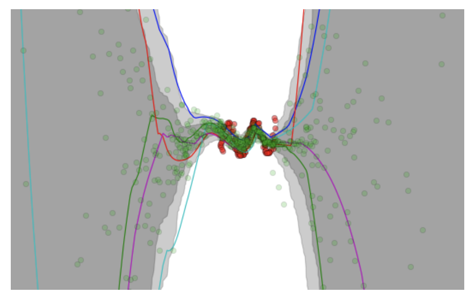
A figure copied from the VIME paper (NIPS 2016) showing Bayesian Neural Network predictions and uncertainty levels.

For instance, in the figure above (taken from the VIME paper) the authors construct a regression task, where the network takes in a scalar-valued⁵ input \(x \in \mathbb{R}\) and outputs a prediction \(y \in \mathbb{R}\). The red dots are the targets, while the green dots are the predictions. It’s clear that the red dots are clustered near the center of the figure, so logically, our Bayesian Neural Networks should be very confident in their predictions in those areas, and less confident outside the training data’s dominant regime. Indeed, the shaded areas confirm this, as they represent the output mean plus/minus one and two standard deviations (I think the second standard deviation is too far to see for the extremes in this figure) based on different neural network weight parameters.

These types of figures are typically shown when people talk about Bayesian Neural Networks, such as in Yarin Gal’s excellent tutorial.

Code Implementation

I am working on implementing Bayesian Neural Networks in my MCMC repository, which is a TensorFlow implementation based on Tianqi Chen’s earlier pure numpy code. The code is a bit disorganized and not quite ready for consumption by the public, but I think I’m getting something going with this code.

---

In this post, I attempt to learn as much as possible about the paper Multi-Level Discovery of Deep Options, which introduced the DDO algorithm. This post is split into my understanding of the math, followed by implementation/experiments.

Before we begin, here is some useful notation:

• Options are denoted as \(h = \langle \pi_h, \psi_h \rangle \in \mathcal{H}\), with \(\mathcal{H}\) representing the set of possible options. To make the notation clearer when we’re dealing with options at each time step \(t\), we could write \(\mathcal{H} = \{h_{\rm opt}^{(1)}, \ldots, h_{\rm opt}^{|\mathcal{H}|}\}\).

• Higher-level policies are denoted as \(\eta(h \mid s)\), in which we pick options. You could also repeat this recursively; think of using something like \(\eta'(\eta \mid s)\), though the paper never officially uses that notation.

• A set of \(K\) demonstrations are denoted as \(\{\xi_1, \ldots, \xi_K\}\). They do not assume that these demonstrations are from an expert supervisor, only that (a) they have some hierarchical structure to be discovered, and (b) that they are informative of the relevant actions to take in each state. Assumption (a) is easier to understand and justify, for if we didn’t have a hierarchical structure to discover, there is no point doing DDO or any hierarchical learning algorithm. Fortunately, in many real-life tasks (for humans), we have hierarchical structures.

The paper also goes through some usual reinforcement learning and imitation learning notation, which I won’t repeat here as it will be clear to those with the relevant background.

The goal of DDO is to discover a set of parameterized options from \(\{\xi_1, \ldots, \xi_K\}\).

The Math

To derive the math, the authors use the perspective of fitting a generative model to the trajectories. That generative model, however, has latent variables, so they need to perform a flavor of Expectation-Maximization, which I’ve previously blogged about here.

But what are the latent (a.k.a., hidden) variables?

• The choice of \(h_t \in \mathcal{H}\), which represents the option at time \(t\).

• In addition, their generative model also assumes that at each time step, we have a binary random variable \(b_t \in \{ 0, 1 \}\), where if \(b_t=1\), a new option is drawn from the high-level policy. The random variable follows a Bernoulli distribution with parameter based on the option termination conditions \(\psi_h\); the higher the value at a given state, the more likely it is that the option should finish and return control to the meta-policy.

The generative model tells us how to assign probabilities to the trajectories. Now, let’s figure out how to find \(\theta \in \Theta\) that maximizes the likelihood of the trajectories! We’re using \(\theta\) to denote all the parameters of everything together: the meta-control policy and for each option. The derivation here assumes a two-level hierarchy, but the extension to multiple levels should be straightforward, besides some nightmarish notation.

The discussion above makes it clear that the \(i\)th trajectory in our data follows this structure:

\[\tau_i = (\underbrace{s_0, a_0, s_1, \ldots, a_{T-1}, s_T}_{\xi_i}, \underbrace{b_0, h_0, b_1, h_1, \ldots, h_{T-1}}_{\zeta_i})\]

with \(\xi_i\) and \(\zeta_i\) representing the visible and latent variables, respectively.

To find parameters, we need to encode this probabilistically, as in \(p(\xi_i, \zeta_i)\). Fortunately, as is standard in RL/IL, this long joint probability decomposes based on time steps. Specifically, we express it as:

\[\mathbb{P}_\theta(\zeta_i, \xi_i) = p_0(s_0) \delta_{b_0=1} \eta(h_0 | s_0) \times \prod_{t=1}^{T-1} q_\theta(b_t,h_t | h_{t-1},s_t) \times \prod_{t=0}^{T-1} \pi_{h_t}(a_t|s_t) p(s_{t+1}|s_t,a_t)\]

where for notational clarity, we denote the various probability distributions as follows:

• \(p_0\) represents the probability distribution over the initial state. There is no dependence on \(\theta\).
• \(p(s' | s,a)\) represents the dynamics of the environment. Once again, there is no dependence on \(\theta\).
• \(q_\theta(b_t,h_t | h_{t-1},s_t)\) represents the distribution over the hidden variables. (My notation is slightly different than what the DDO paper uses, but I find it easier to think of the entire likelihood \(\mathbb{P}_\theta\) as distinct from this.)
• \(\pi\) and \(\eta\), of course, represent the policy and option selection.

Since \(b\) is Bernoulli, we can easily split \(q_\theta\) into cases to define it more precisely:

\[q_\theta(b_t=0,h_t \mid h_{t-1},s_t) = (1-\psi_{h_{t-1}}(s_t)) \cdot \delta_{h_t=h_{t-1}}\]

and

\[q_\theta(b_t=1,h_t \mid h_{t-1},s_t) = \psi_{h_{t-1}}(s_t)\cdot \eta(h_t|s_t)\]

We should now step back and ask ourselves if this definition of \(\mathbb{P}_\theta(\zeta_i, \xi_i)\) makes sense. Does it?

Yes. The first few terms draw the initial state, and then the \(\delta_{b_0=1}\) ensures that we actually have an option to sample from to start (though it is really unnecessary notation). Then we assume we draw \(h_0\).

Next, we iterate through the remaining time steps. We draw the action based on the policy, and then the dynamics provide the state. But then we also need to sample the two latent variables. We’re packing these together in \(q_\theta\), but you can also think of it sequentially: first sampling a Bernoulli for the option termination, and then sampling from the meta-policy. The split of \(q_\theta\) in two cases makes the sequential aspect of this clearer: \(\psi_{h_{t-1}}\) represents the probability that \(b_t=1\), and if it is zero (with probability \(1-\psi_{h_{t-1}}\)), we don’t need to draw at all, hence the delta term \(\delta_{h_t=h_{t-1}}\). Otherwise, we need to sample, hence the \(\eta(h_t|s_t)\). Yes, this all makes sense, and can be reasoned by iterating through the generative model “pseudocode.”

Great. Now we know the likelihood of one trajectory. We want to maximize the (log) likelihood \(L(\theta | \xi)\) assigned to a trajectory, which means we need to take gradient steps to get our neural network weights to go to the correct spot. For one trajectory \(\xi\) (omitting the subscript which normally indicates which trajectory in our set of them), we have:

\[\begin{align} \nabla L(\theta | \xi) \;&{\overset{(i)}{=}}\; \nabla_\theta \log \mathbb{P}_\theta(\xi) \\ \;&{\overset{(ii)}{=}}\; \frac{1}{\mathbb{P}_\theta(\xi)} \sum_{\zeta \in (\{0,1\} \times \mathcal{H})^T} \nabla_\theta \mathbb{P}_\theta (\zeta, \xi) \\ \;&{\overset{(iii)}{=}}\; \sum_{\zeta} \frac{\mathbb{P}_\theta(\zeta, \xi)}{\mathbb{P}_\theta(\xi)} \cdot \nabla_\theta \log \mathbb{P}_\theta(\zeta, \xi) \\ \;&{\overset{(iv)}{=}}\; \sum_{\zeta} \mathbb{P}_\theta(\zeta | \xi) \cdot \nabla_\theta \log \mathbb{P}_\theta(\zeta, \xi) \\ \;&{\overset{(v)}{=}}\; \mathbb{E}_{\zeta | \xi ; \theta}\big[\nabla_\theta \log \mathbb{P}_\theta(\zeta, \xi) \big], \\ \;&{\overset{(vi)}{=}}\; \mathbb{E}_{\zeta | \xi ; \theta}\left[ \nabla_\theta \log \eta(h_0 | s_0) + \sum_{t=1}^{T-1}\nabla_\theta \log q_\theta (b_t,h_t | h_{t-1},s_t) + \sum_{t=0}^{T-1} \nabla_\theta \log \pi_{h_t}(a_t | s_t) \right], \end{align}\]

Where in (i) we substituted the definition with the thing we want to optimize since that will lead to “likely” trajectories learned from gradient steps, in (ii) we applied the \(\nabla \log p(x) = \frac{\nabla p(x)}{p(x)}\) “trick” and then applied the probability 101 rule that \(p(x) = \sum_z p(x,z)\) while explicitly writing out what it means to sum over the discrete-valued \(\zeta\) latent variable over all \(T\) times (this is an exponentially large sum!), in (iii) we again applied the same log-derivative trick, except this time from the perspective of \(\nabla p(x) = p(x) \nabla \log p(x)\), in (iv) we used the definition of conditional probability and then the definition of expectation in (v), and finally in (vi) we applied our previous derivation of the probability of both the visible and latent variables, and omitted terms which cancel out from the gradient. Recall again that \(\theta\) includes the parameters of the meta policy (i.e., \(\eta\)) and the lower-level options \(h_t \in \mathcal{H}\).

In general, we’re dealing with a batch of trajectories, so just apply it to each of the trajectories and take an average over the minibatch to make the gradient independent of batch size.

This is good, but we can actually write the gradient more explicitly, without the expectation by converting the expectation to the sums. Effectively, instead of doing the step (vi) to (v) thing we did earlier, we’ll explicitly simplify the probability based on the summation. However, we’ll start from step (vi) above since it’s easier to manage the calculations with all the stuff canceled out after applying \(\nabla_\theta\). We’ll go through this computation in several steps.

For the third term, we have:

\[\begin{align} \mathbb{E}_{\zeta | \xi ; \theta}\left[ \sum_{t=0}^{T-1} \nabla_\theta \log \pi_{h_t}(a_t | s_t) \right] \;&{\overset{(i)}{=}}\; \sum_{t=0}^{T-1} \mathbb{E}_{\zeta | \xi ; \theta} \Big[ \nabla_\theta \log \pi_{h_t}(a_t|s_t)\Big] \\ \;&{\overset{(ii)}{=}}\; \sum_{t=0}^{T-1} \mathbb{E}_{h_t | \xi; \theta} \Big[ \nabla_\theta \log \pi_{h_t}(a_t|s_t) \Big] \\ \;&{\overset{(iii)}{=}}\; \sum_{h \in \mathcal{H}} \sum_{t=0}^{T-1} \mathbb{P}_\theta(h_t=h | \xi) \cdot \nabla_\theta \log \pi_{h_t}(a_t|s_t). \end{align}\]

Where (i) is by linearity of expectation, (ii) simplifies the expectation by realizing that the term under expectation only (directly) depends on \(h_t\), and (iii) applies the definition of expectation. If step (ii) isn’t clear, it should work out if you expand the full probability into sums over all \(h_t\) and all \(b_t\). Then the \(b_t\) sums should get “pushed to the right” and sum to one (and thus go away) and the rest should follow from there. I would write it out, except that it makes sense to me and I don’t want to spend my entire blogging career getting bogged down with notation.

Additional comment: it might also be the case that conditioning on \(\xi\) instead of just the relevant part of \(\xi\) was done for notational convenience.

Next, here’s how to rewrite the first two terms in the expectation. This requires a considerable amount of care:

\[\begin{align} & \mathbb{E}_{\zeta | \xi ; \theta}\left[ \nabla_\theta \log \eta(h_0 | s_0) + \sum_{t=1}^{T-1}\nabla_\theta \log q_\theta (b_t,h_t | h_{t-1},s_t) \right] \\ &= \mathbb{E}_{\zeta | \xi ; \theta}\Big[ \nabla_\theta \log \eta(h_0 | s_0)\Big] + \sum_{t=1}^{T-1} \mathbb{E}_{\zeta | \xi ; \theta} \Big[\nabla_\theta \log q_\theta (b_t,h_t | h_{t-1},s_t) \Big] \\ &= \mathbb{P}_\theta(b_0=1,h_0=h)\nabla_\theta \log \eta(h_0 | s_0) + \sum_{t=1}^{T-1} \mathbb{E}_{h_{t},b_t| \xi ; \theta} \Big[\nabla_\theta \log q_\theta (b_t,h_t | h_{t-1},s_t) \Big] \\ &= \mathbb{P}_\theta(b_0=1,h_0=h)\nabla_\theta \log \eta(h_0 | s_0) + \sum_{t=1}^{T-1} \sum_{h \in \mathcal{H}} \mathbb{P}_\theta(b_t=0,h_t=h|\xi) \nabla_\theta \log(1-\psi_{h_{t-1}}(s_t)) + \mathbb{P}_\theta(b_t=1,h_t=h|\xi) \nabla_\theta \Big[ \log \psi_{h_{t-1}}(s_t) + \log \eta(h_t|s_t) \Big] \\ &= \sum_{h \in \mathcal{H}} \left[ \left\{ \sum_{t=0}^{T-1} \mathbb{P}_\theta(b_t=1,h_t=h | \xi) \cdot \nabla_\theta \log \eta(h_t|s_t)\right\} + \left\{ \sum_{t=1}^{T-1} \mathbb{P}_\theta(b_t=0,h_t=h | \xi) \cdot \nabla_\theta \log (1-\psi_{h_{t-1}}(s_t)) + \mathbb{P}_\theta(b_t=1,h_t=h | \xi) \cdot \nabla_\theta \log (\psi_{h_{t-1}}(s_t)) \right\} \right]\\ \end{align}\]

For the most part, it uses similar techniques as the other part, such as converting the expectation to sums over probabilities (i.e., applying the definition) and then moving the sums to the right as far as possible so that they can sum to one and then eliminate. The main challenge here is tracking all the \(b_t\)s here in addition to the \(h_t\)s.

Putting all this together, we get the equation shown in the DDO paper where they’ve substituted in \(u_t(h), v_t(h)\), and \(w_t(h)\) terms. It should be equivalent to what I have above, though the odds that there is a typo somewhere (probably above) is 100 percent. I think I know how this works in theory but there is a lot of notation.

Incidentally, there is some good explanation about how — since we’re living in discrete-land — there are three cross entropy loss terms embedded into the gradient update.

The last piece of math to note before proceeding to the implementation details is … how to implement Expectation-Gradient efficiently. Fortunately, the Expectation step — where latent variables are “sampled” and weighted probabilistically — can be done with the Baum-Welch update, which I have previously blogged about. I won’t go through the details here, though I went through them on pencil and paper and the math makes sense. The key to my intuition is to think of forward and backward probabilities as “counting up” the number of ways to reach a given spot from the start (for trajectory prefixes) or the end (for trajectory suffixes). The Baum-Welch algorithm gives us efficient ways to compute various probabilities, and then, since we can formulate a loss function which is the negative log likelihood of a trajectory, we can call TensorFlow to compute gradients for us for the Gradient step. Thus, we have the Expectation-Gradient algorithm.

Quick note: recall Expectation-Maximization. They’re not doing that because the maximization part can’t be done in closed form with neural network models:

Our work is most related to [43], who use a similar generative model, originally introduced by [8] as an Abstract Hidden Markov Model, and learn its parameters via the Expectation-Maximization (EM) algorithm. EM applies the same forward-backward E-step as our Expectation-Gradient algorithm (Section 4.2) to compute marginal posteriors, but uses them for a complete optimization M-step over the options and the meta-control policies. This optimization is infeasible for expressive representations, as well as for multi-level hierarchies.

OK, now let’s move on to some of the implementation details and experimental results.

Implementation Details and Experiments

I am mostly going to investigate their GridWorld-related experiments, as the Atari stuff uses RAM, not images, so it’s hard to interpret, and the surgical robotics part is impossible to comprehend without intimate knowledge of the training data.

They consider DDO under two different scenarios:

(Supervised) given a supervisor who demonstrates a few times how to perform a task, show that the discovered options are useful for accelerating reinforcement learning on the same task; (Exploration) apply reinforcement learning for \(T\) episodes, sample trajectories from the current best policy, and augment the action space with the discovered options for the remaining \(T'\) episodes

This is a bit confusing to me for a few reasons. I will state why later when I review some questions I have about the paper. Let’s move on to GridWorld. Details:

• a \(15 \times 11\) grid, with four rooms.
• the agent actions is randomized with probability 0.3.
• the agent can move in four directions (the “atomic actions”), and moving into wall has no effect.
• an apple is spawned in random location, and upon reaching it the agent gets +1 reward (and then it is respawned).
• the agent knows where it is, as it’s hard-coded in the state space.

All neural network policies (for control, meta-control, termination) are neural nets with one hidden layer of … two nodes. Yeah, you don’t need much for GridWorld.

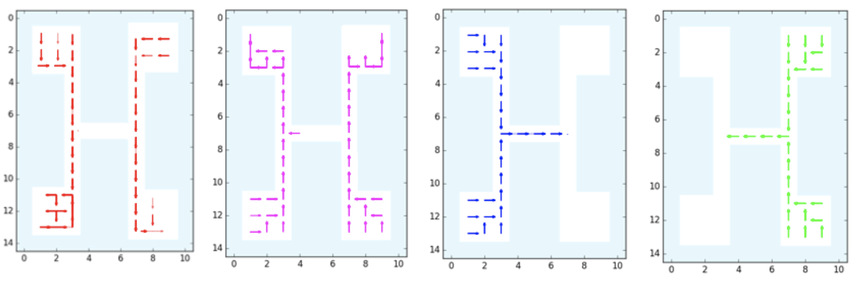The GridWorld used in the DDO paper. It is repeated four times in this image, each with a different discovered option: down, up, right, and left, respectively.

For the two setups:

• Supervised. They generate 50 trajectories of length 1000 using Value Iteration. (1000 seems like a large number, but the agent repeatedly respawns after hitting the apple so trajectories can go on indefinitely.) Then, after running DDO on this data, they can discover options. This is the supervised case, so there is (I assume) no environment interaction during the DDO stage. They executed the learned options and found four of them at the lower level (see figure above). There’s another figure for the higher-level options, which shows the options that are invoked to move the agents to rooms, starting from any given state.

• Exploration. They trained a DQN agent for 2000 steps with atomic actions. Then after those steps, they can roll out trajectories from the \(\epsilon\)-greedy policy, which effectively turn this into a “supervised” case. DDO learns options, and then the Q-function is then reset and DQN is run again with the augmented action space. I think what they want to show is that, compared to baseline DQN, the DQN augmented with options learns faster. It is a little hard to interpret Figure 2, though. They are starting from 2000 steps when they compute the number of steps for the option-augmented agents, right? (Because that’s 2000 steps of computation needed.) I think so, as their Figure 2 plots for the “exploration setting” are like the ones from the “supervised” setting except shifted to the right past 2000 steps, but then I’m surprised at why rewards shoot up at (essentially) exactly 2000 steps.

I also read through their Supplementary Material, which provides mostly more information on various GridWorld settings. Figure 7 appears to be missing the benchmark of having options-only DQN, but otherwise it has primitives-only DQN and options-and-primitives DQN, which is the “augmented DQN” from the paper.

Now here are some questions I have:

• For the supervised setting of DDO, is it fair to say it “accelerates RL”? In the default RL setting, we do not start with expert trajectories. Thus, any time we can get expert trajectories to bootstrap our starting policy, isn’t that an unfair advantage? This is what I wondered about when digesting the first half of Figure 2. Perhaps the comparison should be with reinforcement learning initialized with behavior cloning?

• For the exploration setting of DDO, what does it mean to augment the action space with discovered options? I think it means this: suppose our default action space is \(\mathcal{A} = \{a_1,a_2,a_3,a_4\}\). Then we discover three options, so the action space becomes \(\mathcal{A}' = \mathcal{A} \cup \{h_{\rm opt}^{(1)}, h_{\rm opt}^{(2)}, h_{\rm opt}^{(3)}\}\). Is that right? Then how is this logic implemented? The original RL policy must have started with a neural network that outputs four components, one per action (so that we can do a softmax to get the full probability distribution). Do we then copy weights over to a new neural network with seven outputs, so that all weights except for the last layer are pre-initialized?

• Regarding the DQN results, DQN is notorious for requiring lots of hyperparameter tuning and there are many ways that the implementation can go wrong. I wonder if this was hand-implemented or if the authors based it on an existing library with known benchmarks.

Whew! That was a fairly exhausting read. I needed to read this three times (which is the amount Professor Michael I. Jordan keeps telling us to read textbooks) but at least I think I get the gist of how DDO works.

Last Friday, I participated in the Bay Area Robotics Symposium for the first time. Since 2013, this has been an annual November event with alternating hosts of the University of California, Berkeley, and Stanford University. This year, it was held in Berkeley, and since by now I am closer to calling myself a robotics researcher, and additionally have (finally!) a robotics-related preprint online, I really had no excuse not to join this time around.

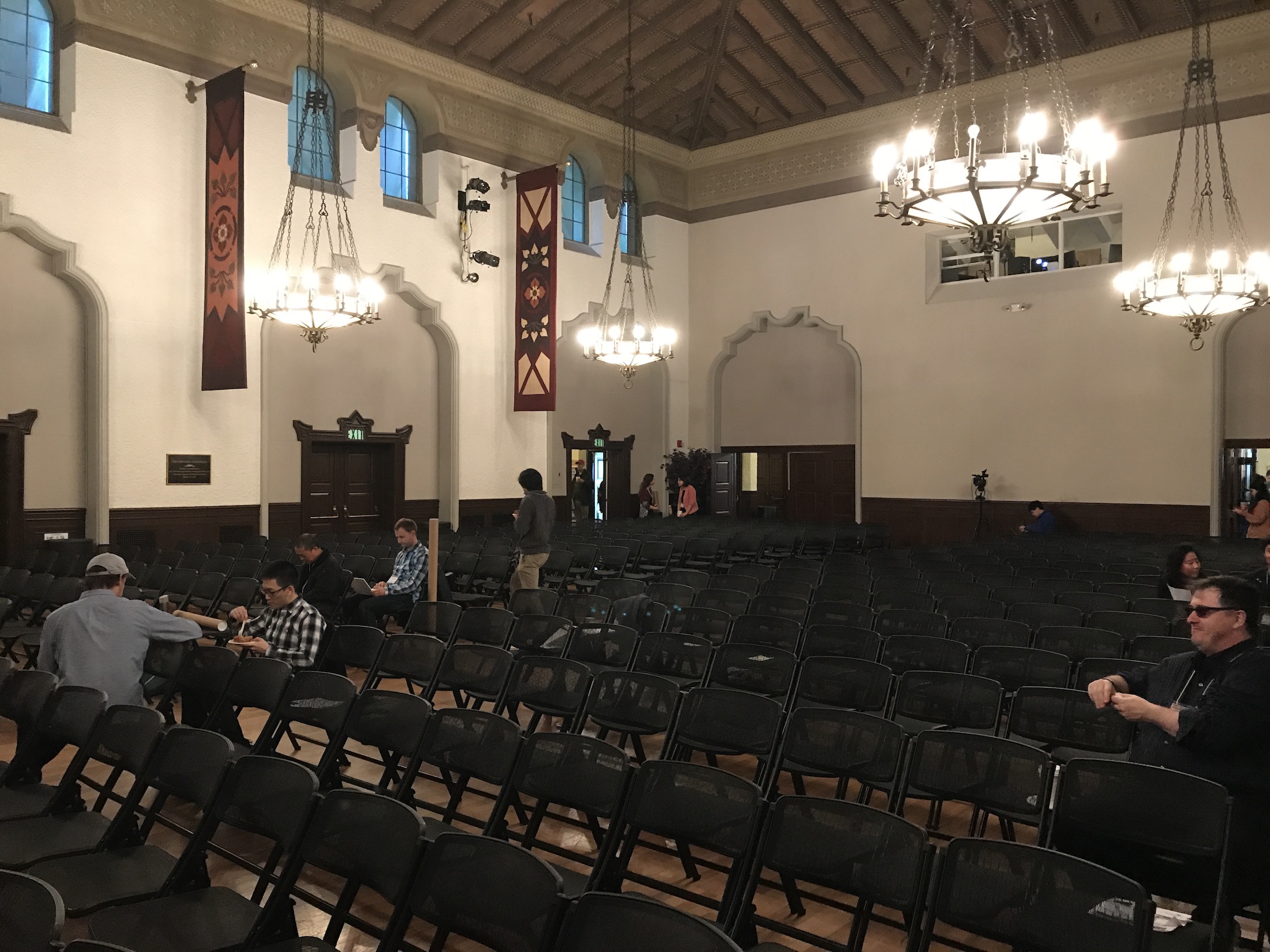The International House auditorium, where BARS took place.

BARS took place at the International House in the southeast corner of the UC Berkeley campus. The talks were in the room shown in the picture above. As usual:

• I arrived early.
• I sat near the front of the room. Thus, this picture shows basically the entirety of the auditorium.

I normally follow the two rules above because of the need to (a) meet my sign language interpreters early, and (b) grab a seat by the front to get a good view of them. Sadly, it means that (as usual) I don’t get other students to sit next to me. In fact, the seats nearby me were empty. One of these days, I will figure out how to sit next to other students.

After about a 15 minute delay (typical Berkeley), BARS finally got started. The Berkeley host, Professor Anca Dragan, gave a few opening remarks, which included that BARS 2017 had (if I recall correctly) 392 people signed up. The capacity was 500, I think, and I’m actually surprised that we didn’t hit the limit. Perhaps CoRL 2017, held recently, meant that BARS 2017 was redundant?

Anyway, soon we started off with the agenda. We started with the first of four sets of faculty talks, each consisting of six faculty giving ten minute talks. Berkeley Professor Pieter Abbeel started things off.

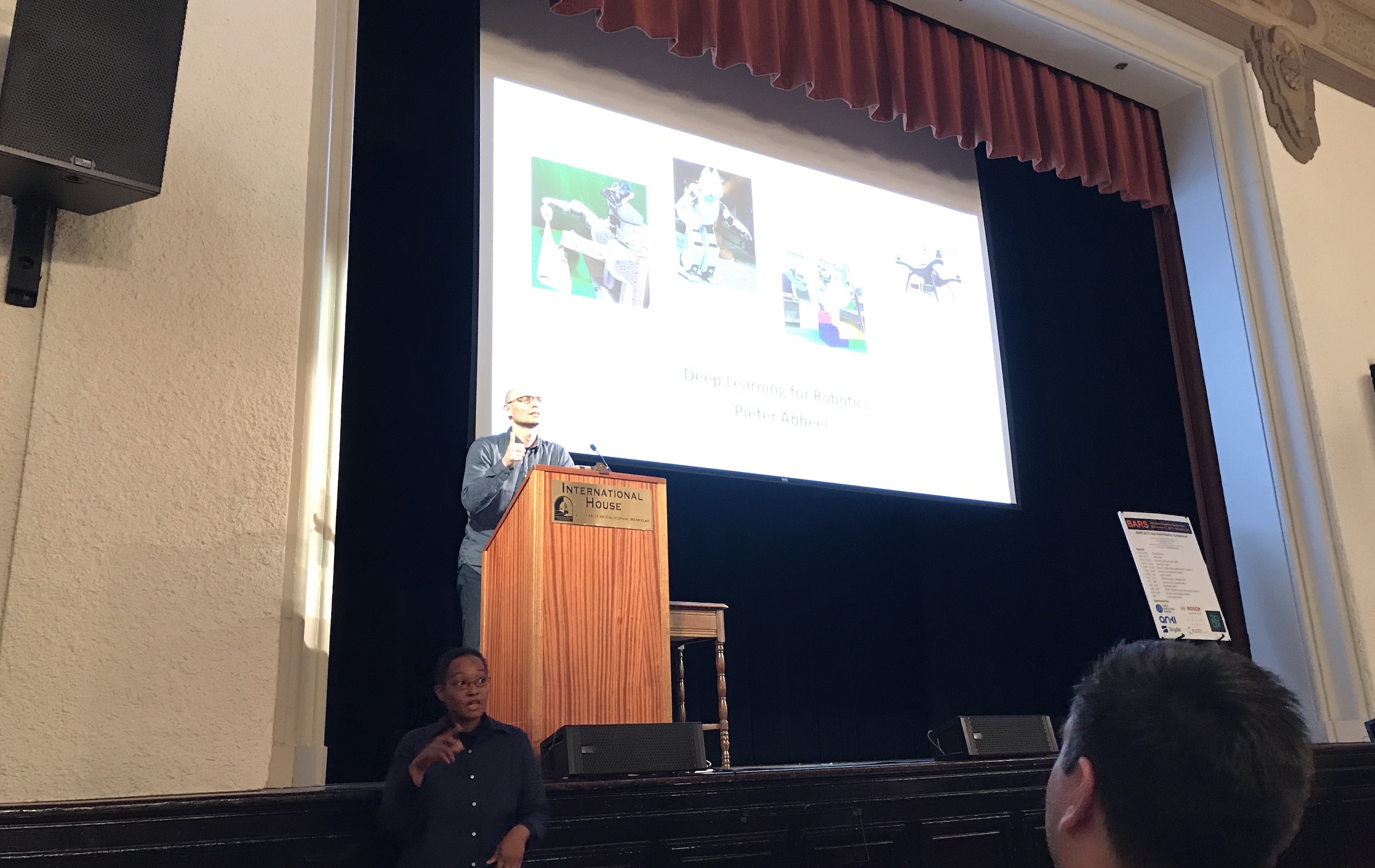Pieter Abbeel started off the faculty talks. He presented "Deep Learning for Robotics". Apologies for the glare on the camera --- I am a rookie with using my iPhone for cameras. You can also see my sign language interpreter there, who had her work cut out for her due to Abbeel's fast and energetic speaking rate.

My goodness, how does he get all these papers?!? His talk started off by listing his long list of publications … in 2017 alone. Then he talked about Meta-Learning, which is what he’s most interested in nowadays within AI. (Just to be clear, I said “most interested,” not “the only thing he’s interested in.”) Incidentally, Abbeel was featured in the New York Times for co-founding Embodied Intelligence. I’m excited to see what they will produce.

We then had more faculty talks. Once these concluded, we moved on to the first of two student spotlight talk sessions, when students gave 1-minute lightning talks on their research. As expected, about 90% of the students went over their alloted time, and most wasted time by saying “My name is X and I’m a student at Y advised by Z and blah blah blah.” The good news is that many of the presentations were interesting enough to pique the curiosity of a nontrivial fraction of the audience. Then those folks can read the students’ papers in their own time.

I didn’t give a lightning talk. I’m not sure why, but I suppose professors could only pick two or three of their students due to time constraints.

We then had our first coffee break. Yay! I stood up, stretched, and briefly chatted with a few other people from Berkeley who I knew. I wish I had talked to some students from Stanford, though. How do people network to brand-new folks at events like these? I really wish I knew the answer.

After another set of faculty talks (including Ken Goldberg’s work on the Dexterity-Network), and then a lunch break, we had … our keynote talk.

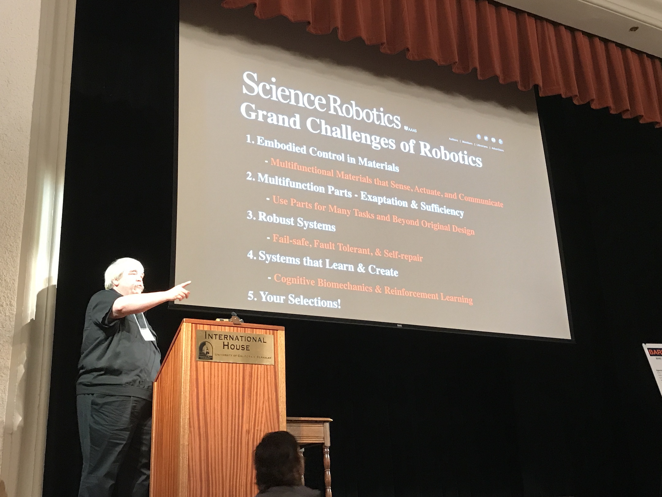Professor Robert Full at the end of his keynote talk, asking the audience about our thoughts on a suitable "Grand Challenge" for robotics.

Professor Full isn’t technically a core robotics faculty — I think — because “biomechanics” is a better way of describing his work. But he quickly captivated the audience with his funny videos on insects and squirrels going through wild motions … and then videos of robots attempting to replicate that movement. I particularly liked the videos of insects and robots that were able to resist insane amounts of forces and squeeze their way through impossibly tiny paths. Judging from the frequent audience laughter, I wasn’t the only one who enjoyed his talk.

Towards the end, Professor Full asked us for “Grand Challenges” of Robotics. One of the professors who I work with, Ken Goldberg, offered “the ability of a robot to pick up anything a human can pick up, including stuff that doesn’t want to be picked up.” You can verify this by looking at his Twitter. I agree with him.

Ken, meanwhile, helped me out a bit later that day. During the second coffee break, Ken gathered a few of his students (including me) and introduced us to Stanford Professor Allison Okamura, who’s also done some work on surgical robotics. At least I got to network a bit, which is better than the usual nothing!

We then had our second set of lightning talks, with the same old issues (people going over their time, etc.), and then our fourth set of faculty talks. This featured stars such as Jitendra Malik and Sergey Levine. I enjoyed Malik’s talk, which was entertaining for two reasons. First, he joked that vision and robotics people (and Malik is a vision person) were historically separate communities in AI, but after drastic improvements in image recognition due to Deep Learning, the “robotics people better pay attention to what the vision people are doing.”

The second joke Malik made was with regards to Stanford vs Berkley. The joke was that Stanford people could develop algorithms for robots (e.g., navigation) that perform well when applied to Stanford-based environments, but which fail on Berkeley-based environments. Why? Stanford is nice and clean, Berkeley is dirty and messy.

Well, UC Berkeley may be a bit run down, not to mention crowded (see image below), but it’s the people that matter, right?

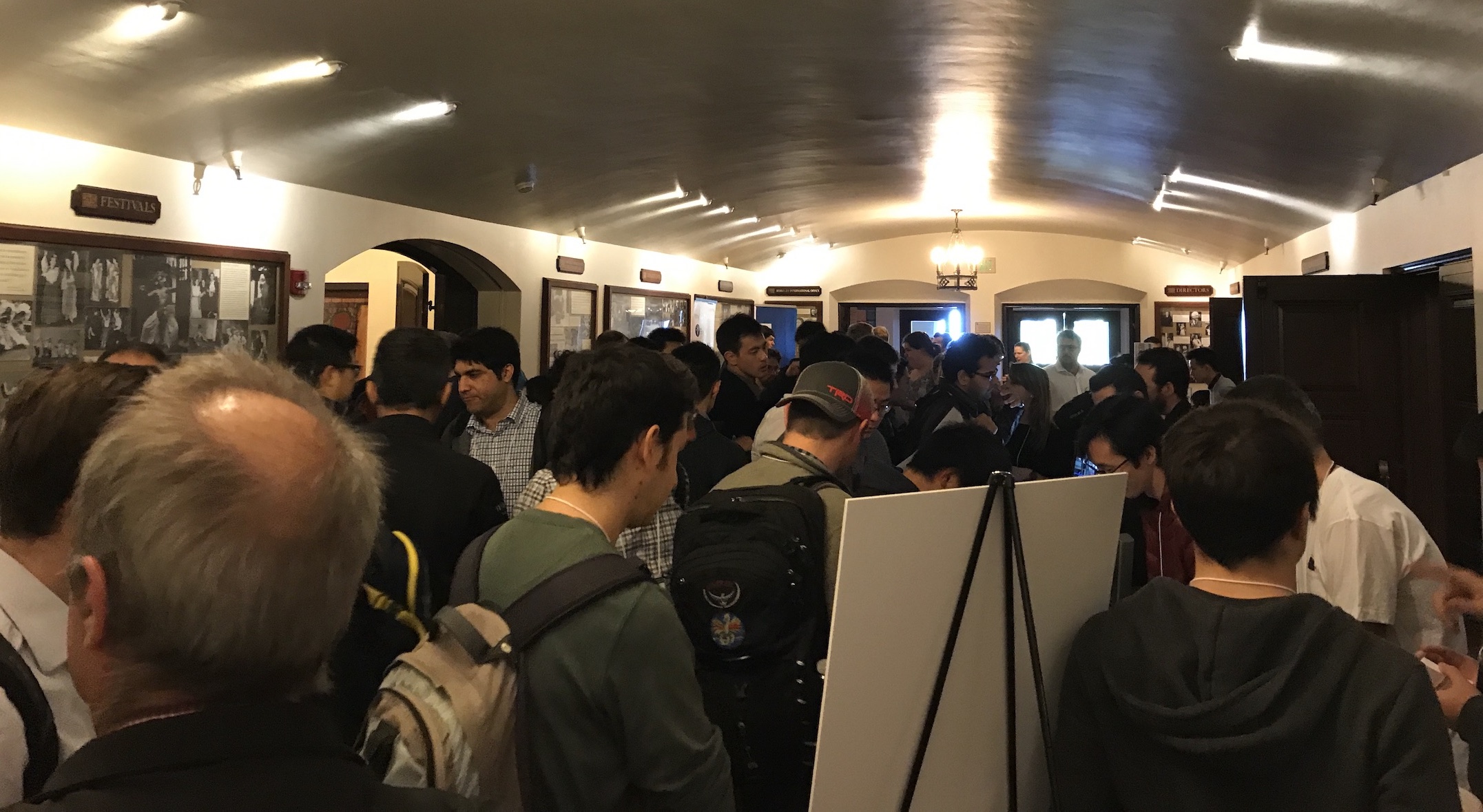Yeowch. BARS sure was popular! Well, that, and the venue is a bit too small for what we're offering. No wonder I regularly hear complaints that Berkeley is too crowded.

Some random, concluding thoughts:

• Two areas of research in robotics (and AI more generally) that are hugely popular are safety and robustness. These are related, though there are subtle differences.

• There were several faculty talking about aerospace dynamics and mechanical engineering. This is not my area of research so I had a hard time processing the concepts. There was also more on surgical robotics than I expected, due to several Stanford faculty (as our surgical robotics person, Ken, is mostly working on grasping). Berkeley, naturally, has more faculty who do Deep Reinforcement Learning for Robotics, and I find that to be the most riveting field of robotics and AI.

• Many faculty kept saying some variant of: “we’ll do Deep Learning because it’s so popular and works.” Yes, I know it’s popular, and it’s funny to talk about it, but by now this has grown stale on me and I wish people would cut back on their hackneyed Deep Learning comments.

• Unfortunately, since I spent most of the coffee breaks talking to a few people or relaxing, I didn’t get to attend either poster session. I got a glimpse of one of them and it looked crowded (and noisy) so maybe I didn’t miss much.

Well, that’s a wrap. I look forward to attending BARS 2018 at Stanford. Thank you to everyone who helped make BARS 2017 happen!

When reading academic papers about a certain subfield, I often find it difficult to clearly understand how they connect with each other. For example, what algorithms are based on other algorithms? Can the contributions of two papers be combined? Would combining them result in notable improvements or just on-the-margin, negligible changes? (The answer to that last question is usually “the latter” but it’s something we should at least consider.)

This post is an attempt to unify my understanding of papers related to scalable Markov Chain Monte Carlo and scalable Metropolis-Hastings. By “scalable,” I refer to the usual meaning of using these algorithms in the large data regime.

These are the papers I’m trying to understand:

• MCMC Using Hamiltonian Dynamics, Handbook of MCMC 2010
• Bayesian Learning via Stochastic Gradient Langevin Dynamics, ICML 2011
• Stochastic Gradient Hamiltonian Monte Carlo, ICML 2014
• Austerity in MCMC Land: Cutting the Metropolis-Hastings Budget, ICML 2014
• Towards Scaling up Markov Chain Monte Carlo: An Adaptive Subsampling Approach, ICML 2014
• Firefly Monte Carlo: Exact MCMC with Subsets of Data, UAI 2014
• On Markov Chain Monte Carlo Methods For Tall Data, JMLR 2017.

(All of them are freely available online.)

First, I’ll briefly discuss why we care about the problem of scalability with MCMC and MH. Then, I’ll group these papers into categories and explain how they are connected to each other. This will then motivate our UAI 2017 paper, An Efficient Minibatch Acceptance Test for Metropolis-Hastings.

Why Markov Chain Monte Carlo?

I’m not going to review MCMC here as you can find many other references, both online and in textbooks. It may help to look at my blog post from June 2016 where I describe the general problem setting. My more recent BAIR Blog post also contains some potentially useful background material.

But why use MCMC at all? Here’s one reason: if we use it to sample some model’s parameter \(\theta\), then the chain of samples \(\{\theta_1, \ldots, \theta_T\}\) should let us quantify useful statistics about properties of interest. Two of these are the expectation and variance of something, which we might apply on the parameter itself. We can estimate (for example) the expectation by taking a sequence of the \(K\) most recent samples (or a subsampled sequence) from our chain \(\{\theta_{T-K+1}, \ldots, \theta_T\}\) and then taking the sample vector-valued expectation. More generally, letting \(f\) be a function of the parameters, we can compute the expectation \(\mathbb{E}[f(\theta)]\) using the expectation of the sampled values \(\{f(\theta_{T-K+1}),\ldots, f(\theta_T)\}\).

We can’t do this if we take stochastic gradient steps, because the samples from SGD are not from the posterior distribution of the parameter. SGD is designed to converge around a single point in the space of possible \(\theta \in \Theta\) values, unlike MCMC methods which are supposed to approximate a distribution, which can then be used for sample estimates of expectations and variances.

My perspective is supported in papers such as the SGLD paper from 2011 (one of the papers I listed above); the authors (Welling & Teh) claim that:

Bayesian methods are appealing in their ability to capture uncertainty in learned parameters and avoid overfitting. Arguably with large datasets there will be little overfitting. Alternatively, as we have access to larger datasets and more computational resources, we become interested in building more complex models, so that there will always be a need to quantify the amount of parameter uncertainty.

So … that’s why we like the Bayesian perspective. These authors are rock-stars, by the way, so I generally trust their conclusions.

I’ll be honest, though: I can’t think of something nontrivial I’ve done in which the Bayesian perspective was that useful to me. In Deep Learning, Deep Imitation Learning, and Deep Reinforcement Learning, I’ve never used priors and posteriors; RMSProp or Adam is good enough, and it seems like this goes for the rest of the community. Maybe it’s just not that necessary in these domains? I have two papers on my reading list, Bootstrapped DQNs and Robust Bayesian Neural Networks, which might clarify some of my questions regarding how much of a Bayesian perspective is needed in Deep Learning. I should also definitely check out the Bayesian Deep Learning NIPS workshop.

Langevin Dynamics and Hamiltonian Dynamics

This section concerns the following three papers:

• MCMC Using Hamiltonian Dynamics, Handbook of MCMC 2010
• Bayesian Learning via Stochastic Gradient Langevin Dynamics, ICML 2011
• Stochastic Gradient Hamiltonian Monte Carlo, ICML 2014

I gave a brief introduction to Langevin Dynamics in my earlier blog post, so just to summarize for this one, Langevin Dynamics injects an appropriate amount of noise so that (in our context) a gradient-based algorithm will converge to a distribution over the posterior of \(\theta\). The Stochastic Gradient Langevin Dynamics algorithm combines the computational efficiencies of SGD by using a minibatch gradient, but uses the Langevin noise to appropriately cover the posterior:

[…] Langevin dynamics which injects noise into the parameter updates in such a way that the trajectory of the parameters will converge to the full posterior distribution rather than just the maximum a posteriori mode.

As a follow-up, the Stochastic Gradient Hamiltonian Monte Carlo (SGHMC) algorithm is similar to SGLD in that it uses a minibatch gradient along with “exploration noise.” This time, the noise is from Hamiltonian Monte Carlo, which is more sophisticated than Langevin Dynamics since HMC introduces extra momentum variables which allows for larger jumps.

Radford Neal’s excellent 2010 book chapter goes over HMC in great detail, so I won’t go through the details here (though I’d like to write a blog post solely about HMC — so stay tuned!). Just to give a quick overview, though, our problem context is similar, where we have a target posterior:

\[p(\theta \mid x_1, \ldots, x_N) \propto \exp(-U(\theta))\]

with potential energy function

\[U(\theta) = -\log p(\theta) - \sum_{i=1}^{N} \log p(x_i \mid \theta).\]

(Don’t worry too much about the “potential energy” terminology; HMC was originally developed from a physics background. We’re still in the same problem setting.)

HMC generates samples from a joint distribution that involves extra momentum variables:

\[\pi (\theta, r) \propto \exp\left(-U(\theta) - \frac{1}{2}r^TMr\right)\]

where \(r\) are the momentum variables and \(M\) is a mass matrix. The update rules are:

• \(\theta = \theta + \tau \cdot M^{-1}r\).
• \(r = r - \tau \cdot \nabla U(\theta)\).

where \(\tau\) is some step size. If this doesn’t make sense, read Neal’s 2010 book chapter.

The result from HMC is a set of samples \(\{(\theta_i,r_i)\}_{i=1}^T\). But we’re only interested in the \(\theta_i\)s, so … we simply drop the \(r_i\) terms to get our samples for \(\theta\). Amazingly, \(\theta\) is sampled from the correct target distribution, which one can show via some “reversibility” analysis.

SGHMC needs a little massaging to actually get it to sample the target distribution, since simply taking a subset of the data to compute an approximation to \(\nabla U(\theta)\) will lose the “Hamiltonian Dynamics” property; the authors resolve this by using second-order Langevin Dynamics to counteract the effect of too much gradient noise in estimating \(\nabla U(\theta)\), and the result is a similar algorithm to SGLD except with a different noise term.

Just to be clear, both SGLD and SGHMC are minibatch, gradient-based algorithms that are also considered “Bayesian methods.” Neither are pure random walks, i.e., neither use Gaussian proposals because the proposals are based on the stochastic gradient value, plus some additive noise term. For SGLD, that extra noise is actually a random walk, but not for SGHMC.

For both SGLD and SGHMC, we have to apply the Metropolis-Hastings test for computer implementations due to discretization error, even though in theory we shouldn’t have to since energy is preserved. In both papers, the authors decrease step sizes to zero so that the MH rejection rate goes to zero. Intuitively, smaller step sizes mean samples are concentrated into higher regions of the posterior, and the gradient ensures going in the direction of greatest increase of the posterior probability. In addition, decreasing step sizes also means discretization error decreases, which yet again further reduces the need for MH tests. While this is great, because the MH test requires full-batch computation, perhaps we are missing out somehow by keeping our step sizes small.¹

Metropolis-Hastings

In this section, I discuss the remaining papers listed at the introduction of this post. They are related in some form to the Metropolis-Hastings algorithm, which is commonly used in MCMC techniques to act as a correction to ensure that samples do not deviate too frequently away from the target posterior distribution.

As I mentioned in both of my earlier blog posts, conventional MH tests require a full pass over the entire dataset. This makes them extremely costly, and is one of the reasons why both SGLD and SGHMC emphasized how decreasing step sizes results in lower discretization error, so that they could omit the MH tests.

Their computational cost has raised the question over whether using subsamples of the data for the MH test computation is feasible. It’s not as straightforward as taking a fixed-sized subset (i.e., minibatch) of the dataset because that results in a non-trivial target distribution which is not the desired posterior.

The following two papers propose subsampling-based algorithms that attempt to tackle the high cost of full-batch MH tests:

• Austerity in MCMC Land: Cutting the Metropolis-Hastings Budget, ICML 2014
• Towards Scaling up Markov Chain Monte Carlo: An Adaptive Subsampling Approach, ICML 2014

I discussed the first one in an earlier blog post. The second one follows a similar procedure as the first one, except that it uses a slightly different way of interpreting when to stop data collection. The downside, as I painfully realized when I tried to implement this, is that due to its concentration bounds, it requires a real-valued parameter which depends on the entire collection of \(\{\log p(x_i\mid \theta), \log p(x_i\mid \theta')\}_{i=1}^N\) values each iteration, which defeats the point of using a subset of the data. (Here, I use \(\theta'\) to denote the proposed distribution.)

The authors of the Adaptive Subsampling paper have a follow-up JMLR 2017 paper (it was under review for a long time) which expands upon this discussion. I found it quite useful, particularly because of their proof (in Section 6.1) about how naive subsampling for the MH test results in a nontrivial and hard-to-interpret target distribution. In Section 6.3, they introduce a novel contribution where they rely on subsampling noise for exploration; that is, use the minibatch-induced noise (which is Gaussian by the Central Limit Theorem) to explore the posterior. However, they showed that this approach still seems to require \(O(n)\) data points each iteration. On the other hand, they didn’t investigate this method in too much detail, so it’s hard to comment on its usefulness.

The last related work was the Firefly paper, which won the Best Paper Award at UAI 2014. It can perform exact MCMC, but the main drawback is (emphasis mine):

FlyMC is compatible with a wide variety of modern MCMC algorithms, and only requires a lower bound on the per-datum likelihood factors.

To be clear on what this means, they require the existence of functions \(B_i(\theta)\) satisfying \(0 \le B_i(\theta) \le p(x_i \mid \theta)\) for all \(i\). How realistic is that? I have no idea, honestly, but it seems like something that is difficult to achieve in practice, especially because it’s conditioning on \(\theta\) and \(\theta'\), which will vary considerably throughout sampling. There is some interesting discussion about this at Christian Roberts’ excellent blog, with Ryan Adams (the professor co-author) commenting.

The prior work then motivated our work, where we avoided needing these assumptions and showed that we could cut the M-H test cost time down to one equivalent with SGD, without loss of performance. There’s no free lunch, though; our algorithm has applicability constraints but those are hopefully not that restrictive. Check out our BAIR blog post for more information.

Conclusion

I’ve discussed these set of papers and tried grouping them together to see a coherent theme in all of this. Hopefully this makes it clearer what these papers are trying to do.

---

In the process of applying to graduate school, and then visiting schools that admitted me, I was told that PhD students needed to possess solid writing ability in addition to technical skills. One UT Austin professor told me he believed liberal arts students (like me) were better prepared than those from large research universities, presumably because of our increased exposure to writing courses. One Cornell professor emphasized the importance of writing by telling me that he spent at least 50 percent of his professional life writing. A Berkeley professor who I frequently collaborate with has a private Google Doc that he gives to students with instructions on writing papers, particularly about how to structure an introduction, what phrases to use, and so on.

The ability to write well is an important skill for academics, and I don’t mean to dismiss this outright. However, I think that we need to be very clear that technical skills matter far, far more for the typical graduate student, at least for computer science students focusing in artificial intelligence like me. I would additionally argue that factors such as research advisors and graduate student collaborators matter more than writing ability.

Perhaps the emphasis on writing skills is aimed at two groups of people: international students, and the very best graduate students for whom technical skills are relatively less of a research bottleneck. I won’t comment too much on the former group, besides saying that I absolutely respect their commitment to learning the English language and that I know I’m incredibly lucky to be a native English user.

I bring up the second group because much of the advice I get are from faculty at top institutions who were stellar graduate students. Perhaps most of their academic life is dominated by the time it takes to convert research contributions to a paper, instead of the time it takes to actually come up with the contribution itself. For instance, this is what UT Austin professor Scott Aaronson had to say in an old 2005 (!!) blog post, back when he was a postdoc (emphasis mine):

I’ll estimate that I spend at least two months on writing for every week on research. I write, and rewrite, and rewrite. Then I compress to 10 pages for the STOC/FOCS/CCC abstract. Then I revise again for the camera-ready version. Then I decompress the paper for the journal version. Then I improve the results, and end up rewriting the entire paper to incorporate the improvements (which takes much more time than it would to just write up the improved results from scratch). Then, after several years, I get back the referee reports, which (for sound and justifiable reasons, of course) tell me to change all my notation, and redo the proofs of Theorems 6 through 12, and identify exactly which result I’m invoking from [GGLZ94], and make everything more detailed and rigorous. But by this point I’ve forgotten the results and have to re-learn them. And all this for a paper that maybe five people will ever read.

Two months of writing for every week of research? I have no idea how that is humanly possible.

For me, the reverse holds: I probably spend two months of research for every week of actual writing. What dominates my academic life is the time it takes (a) to process the details from academic papers so that I understand how their ideas work, and (b) to build upon those results with my own novel contribution. Getting intuition on novel artificial intelligence concepts takes a considerable amount of mathematical thinking, and getting them to work in practice requires programming skills. Both math and programming fall under the realm of “technical skills.”

Obviously, once I HAVE a research contribution, then I have to “worry” about writing it, but I enjoy writing so it is no big deal.

But again, the research contribution itself must first exist. That’s what frustrates me about much of the academic advice that I see. Yes, it’s easier to tell someone how to write (use this phrase, don’t use this phrase, active instead of passive, blah blah blah), but it would be better to explain the thought process on how to come up with an original research contribution.

I conclude:

I would happily trade away some of my writing ability for a commensurate increase in technical skill.

Again, I am not disregard writing ability, since it is incredibly valuable for many reasons (such as for blogging!!) and more applicable than technical skills in life. However, I believe that the biggest priority for computer science doctoral students should be to focus on technical skills.

I first heard about the paper Learning to Act by Predicting the Future after one of the authors, Vladlen Koltun, came to give a highly entertaining talk as part of Berkeley’s Deep Learning seminar course (CS 294-131).

In retrospect, I’m embarrassed it took me this long to find out about the work. It’s research that feels highly insightful and should have been clear to us all along — yet somehow we never saw it until those authors presented it to us. To me, that’s an indicator of high-caliber research.

Others have agreed. Learning to Act by Predicting the Future was accepted as an oral presentation at ICLR 2017, meaning that it was one of the top 15 or so papers. You can check out the favorable reviews on OpenReview. It was also featured on Adrian Colyer’s blog. And of course, it was featured in my Deep Learning class.

So what is the research contribution of the paper? Here’s a key passage in the introduction which explains their framework:

Our approach departs from the reward-based formalization commonly used in RL. Instead of a monolithic state and a scalar reward, we consider a stream of sensory input \(\{s_t\}\) and a stream of measurements \(\{m_t\}\). The sensory stream is typically high-dimensional and may include the raw visual, auditory, and tactile input. The measurement stream has lower dimensionality and constitutes a set of data that pertain to the agent’s current state.

To be clear, at each time \(t\), we get one sensory input and one set of (scalar-valued) measurements, so our observation is \(o_t = \langle s_t, m_t \rangle\). Their running test platform in the paper is the first-person shooter Doom environment, so \(s_t\) represents images and \(m_t\) represents attributes in the game such as health and supply levels.

This is an intuitive difference between \(s_t\) and \(m_t\). There are, however, two important algorithmic differences:

• Given actions taken by the agent, they attempt to predict \(m_t\), hence “predicting the future”. It’s very hard to predict full-blown images, but predicting (much-smaller) measurements shouldn’t be nearly as challenging.

• The measurement vector \(m_t\) is used to shape the agent’s goals. They assume the agent wants to maximize

  \[u(f;g) = g^\top f\]

  where

  \[f = \langle m_{t+\tau_1}-m_t, \ldots, m_{t+\tau_n}-m_t\rangle\]

  Thus, the goal is to maximize this inner product of the future measurements and a parameter vector \(g\) weighing the relative importance of each terms. Note that this instantly generalizes the case with a scalar reward signal in MDPs: we’d set the elements of \(g\) such that they are \(\gamma^0, \gamma^1, \gamma^2, \ldots\), i.e. corresponding to discounted rewards. (I’m assuming that \(m_t\) is a scalar here, but this generalizes to the vector case with \(f\) a matrix, as we could flatten \(f\) and \(g\).)

In order to predict \(m_t\), they have to train a function to do so, which they parameterize with (you guessed it) deep neural networks. They define the function \(F\) as the predictor, with

\[p_t^a = F(o_t, a_t, g ; \theta)\]

Thus, given the observation, action, and goal vector parameter, we can predict the resulting measurements, so that during test-time applications, \(p_t^a\) is “plugged in” for \(f\) and the action which maximizes \(u\) is chosen. To make this work mathematically, of course, \(f,g,\) and \(p_t^a\) must all have the same dimension. And to be clear, even though the reward (as they define it) is a function of \(g\), we are not “training” the \(g\) parameters but the parameters for \(F\).

The parameters of \(F\), incidentally, are trained in an unsupervised manner, or using “self-supervision” since the labels can be generated automatically by having the agent wander around in the world and then repeatedly computing the value of the function output at each of those time steps. Then, after some time has passed, we simply minimize the \(L_2\) loss. Nice, no humans needed for labeling! When I was reading this, I was reminded of the Q-learning update, since the update rule automatically assumes that the “target” is the usual “reward plus discounted max Q-value” thingy, without human intervention. To further the connection with Q-learning, they use an experience memory in the same way as the DQN algorithm used experience replay (see my earlier blog post about DQN). Another concept that came to mind was Sergey Levine’s excellent paper on learning hand-eye coordination, where he and his collaborators were able to automatically generate labels. I need to figure out how to do stuff like this more often.

Anyway, given that \(F\) takes in three inputs, one would intuitively expect that it has three separate input networks and concatenates them at some point. Indeed, that’s what they do in their network, shown below.

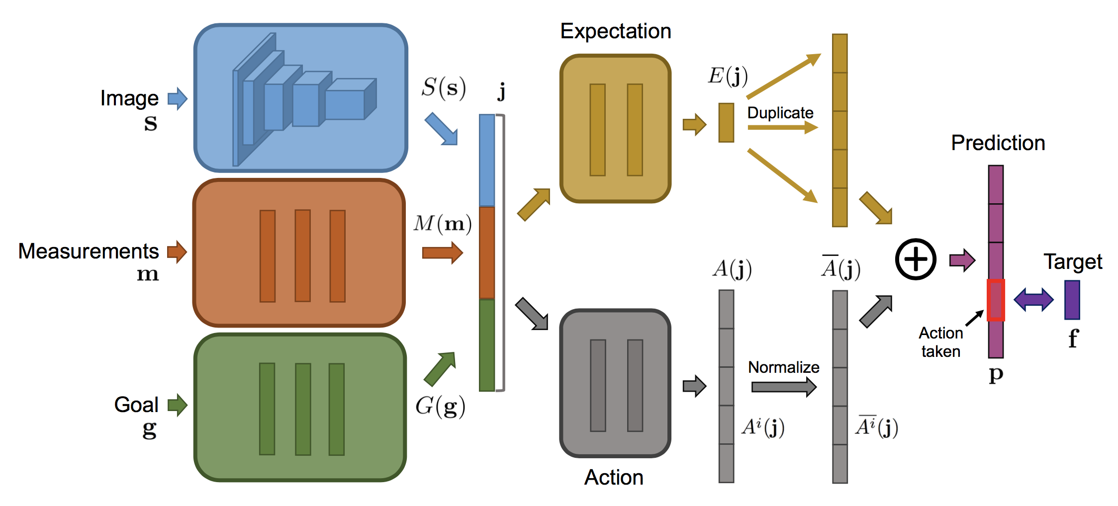
After concatenation, the network follows the paradigm of the Dueling DQN architecture by having separate expectation and value (“action”) streams. It might not be clear why this is useful, so if you’re puzzled, I recommend reading the Dueling DQN paper for justification (I need to re-read that as well).

They benchmark their paradigm (called DFP for “Direct Future Prediction”) on Doom with four scenarios of increasing difficulty. The baselines are the well-known DQN and A3C algorithms, along with a relatively obscure “DSR” algorithm (but which used the Doom platform, facilitating comparisons). I’m not sure why they used DQN instead of, say, Double DQN or prioritized variants since those are assumed to be strictly better, but at least they test using A3C which as far as I can tell is on par with the best DQN variants. It’s too bad that OpenAI baselines wasn’t around in time for the authors to use it for this paper.

They say that

We set the temporal offsets \(\tau_1, \ldots, \tau_n\) of predicted future measurements to 1, 2, 4, 8, 16, and 32 steps in all experiments. Only the latest three time steps contribute to the objective function, with coefficients \((0.5, 0.5, 1)\).

I think they say this to mean that their goal vector \(g\) contains only three nonzero components, corresponding to \(\tau_{n-2}, \tau_{n-1}\) and \(\tau_n\). But then I’m confused: why do they need to have all the other \(\tau_i\) for \(1 \le i \le n-3\)? What’s also confusing is that for the two complicated environments with ammo, health, and frags, their training is set to maximize a linear combination of those three, with coefficients \((0.5, 0.5, 1.0)\). The same vector is repeated here!

I wish they had expanded upon their discussion since this is new stuff from their paper. Why did they choose this and that value? What is the intuition? I know it’s easy to ask this from a reading/reviewing perspective, but that’s only because the concept is new; for example, they do not need to justify why they chose the dueling-style architecture because they can refer to the Dueling DQN paper.

Regarding experiments, I don’t have much intuition on the vizDoom environments, as I have never used those, but their results look impressive on the two harder scenarios, which also provide more measurements (three instead of one). Their method out-performs sophisticated baselines in various settings, including those from the Visual Doom AI competition in September 2016.

At the end of the experimental section, after a few ablation studies (heh, my favorite!) they convincingly claim that

This supports the intuition that a dense flow of multivariate measurements is a better training signal than a scalar reward.

In my words: dense signals are better than sparse signals. In some cases, sparsity is desirable (e.g. in attention models, we want sparsity to focus on a few important components) but for rewards in reinforcement learning, we definitely need dense signals. Note that getting such signals wouldn’t be possible if the authors kept clinging to the usual MDP formulation. Indeed, Koltun made it a point in his talk to emphasize how he disagreed with the constraints imposed on us by the MDP formulation, with the usual “set of states, actions, rewards […]”. This is one of the things I wish I was better at: identifying certain gaps in assumptions that everyone makes, and trying to figure out where we can improve them.

That’s all I have to say for this paper now. For more details, I would check the paper website. Have fun!

Last night, I finished reading Dale Carnegie’s book How to Win Friends and Influence People: The Only Book You Need to Lead You to Success. This is the 31st book I’ve read in 2017, and hopefully I will exceed the 38 books I read in 2016.

Carnegie’s book is well-known. It was originally published in 1936 (!!) during the Great Depression, but as the back cover argues, it is “equally valuable during booming economies or hard times.” I read the 1981 edition, which updated some of the original material to make it more applicable to the modern era. Even though it means the book loses its 1936 perspective, it’s probably a good idea to keep it updated to avoid confusing the reader, and Carnegie — who passed away in 1955 — would have wanted it. You can read more about the book’s history on its Wikipedia page.

So, is the book over-hyped, or is it actually insightful and useful? I think the answer is yes to both, but we’ll see what happens in the coming years when I especially try to focus on applying his advice. The benefit of self-help books clearly depends on how well the reader can apply it!

I don’t like books that bombard the reader with hackneyed, too-good-to-be-true advertisements. Carnegie’s book certainly suffers from this, starting from the terrible subtitle (seriously, “The Only Book”??). Now, to be fair, I don’t know if he wrote that subtitle or if it was added by someone later, and if it was 1936, it would have definitely been more original. Certainly in the year 2017, there is no shortage of lousy self-help books.

The good news is that once you get beyond the hyped-up advertising, the actual advice in the book is sound. My summary of it: advice that is obvious, but that we sometimes (often??) forget to follow.

Indeed, Carnegie admits that

I wrote the book, and yet frequently I find it difficult to apply everything I advocated.

This text appears in the beginning of a book titled “Nine Suggestions to Get the Most Out of This Book”. I am certainly going to be following those suggestions.

The advice he has is split into four rough groups:

• Fundamental Techniques in Handling People
• Six Ways to Make People Like You
• How to Win People to Your Way of Thinking
• Be a Leader: How to Change People Without Giving Offense or Arousing Resentment

Each group is split into several short chapters, ending in a quick one-phrase summary of the advice. Examples range from “Give honest and sincere appreciation” (first group), “smile” (second group), “If you are wrong, admit it quickly and emphatically” (third group), and “Talk about your own mistakes before criticizing the other person” (fourth group). Chapters contain anecdotes of people with various backgrounds. Former U.S. Presidents Washington, Lincoln, and both Roosevelts are featured, but there are also many examples from people leading less glamorous lives. The examples in the book seem reasonable, and I enjoyed reading about them, but I do want to point out the caveat that some of these stories seem way too good to be true.

One class of anecdotes that fits this criteria: when people are able to get others to do what they want without actually bringing it up! For example, suppose you run a business and want to get a stubborn customer to buy your products. You can ask directly and he or she will probably refuse, or you can praise the person, show appreciation, etc., and somehow magically that person will want to buy your stuff?!? Several anecdotes in the book are variants of this concept. I took notes (with a pencil) to highlight and comment in the book as I was reading it, and I frequently wrote “I’m skeptical”. Fortunately, many of the anecdotes are more realistic, and the advice itself is, as I mentioned before, accurate and helpful.

I have always wondered what it must be like to have a “normal” social life. I look at groups of friends going out to meals, parties, and so forth, and I repeatedly wonder:

• How did they first get together?
• What is their secret to liking each other??
• Do I have any ounce of hope of breaking into their social circle???

Consequently, what I most want to get out of the book is based on the second group, how to make people like me.

Unfortunately, I suffer from the social handicap of being deaf. While talking with one person usually isn’t a problem, I can’t follow conversations with noisy backgrounds and/or with many people. Heck, handing a conversation with two other people is often a challenge, and whenever this happens, I constantly fear that my two other “conversationalists” will talk to themselves and leave me out. And how on earth do I possibly network in noise-heavy academic conferences or workshops??? Gaaah.

Fortunately, what I find inspiring about Carnegie’s advice is that it is generic and highly applicable to the vast majority of people, regardless of socioeconomic status, disability condition, racial or ethnic background, and so forth. Obviously, the benefit of applying this advice will vary depending on people’s backgrounds, but for the vast majority of people, there should be some positive, non-zero benefit. That is what really counts.

I will keep How to Win Friends and Influence People on my desk as a constant reminder for me to keep applying these principles. Hopefully a year from now, I can look back and see if I have developed into a better, more fulfilled man.

"No one is born hating another person because of the color of his skin or his background or his religion..." pic.twitter.com/InZ58zkoAm

— Barack Obama (@BarackObama) August 13, 2017

President Trump, you should have clearly and unequivocally denounced racism and white supremacy immediately, without trying to pin the blame on “both sides” or whatever other un-related group comes to mind. Your delayed statement does not redeem yourself. It should be easy and automatic to condemn and call out white supremacist groups like the Ku Klux Klan and neo-Nazis. I never thought I would see a current United States President who is afraid to do so.

America has come a long way since the days of George Washington, Abraham Lincoln, and Martin Luther King Jr., but we still have lots of progress to go before we can truly claim that America provides an equal playing field for its citizens.

In the past, I have always told people that I would never use Twitter. I eventually had to sign up to test some features for the BAIR blog since the posts there are “tweeted” via the BAIR Twitter account. I was going to disable my account now that these tests are done, but then I saw the lovely tweet by former President Obama above. I hit “like” on it, and will keep my account active for that reason only. I hope it will remain the most liked tweet forever.

Day Five

Today, August 15, was the last day of UAI 2017. We had workshops, which you can think of as one-day conferences with fewer people. UAI 2017 offered three workshops, and I attended the Bayesian Modeling Applications Workshop. It was a small workshop with only ten of us present at the 9:00am starting time, though a few more would trickle in during the first hour.

Here were some of the highlights:

• David Poole from the University of British Columbia gave the opening talk on Probabilistic Reasoning with Complex Heterogeneous Observations and Applications in Geology and Medicine. This one was largely about ontologies. Unfortunately, in the interest of time, he had to skip a lot of the content.

• The other talks were more directly related to Bayesian networks, which I studied a lot in undergrad and also for my AI prelim exams.

• There was another talk about OpenMarkov. I got mostly distracted when the speaker emphasized the advantage that the software was open source. Maybe this is me coming from Deep Learning, but open source should be the expectation, not the norm. (MuJoCo is the one exception for Deep Learning, but hopefully that will soon no longer be the case.) I was reminded of Zack Lipton’s blog post on a sober perspective of Tensorflow when he wrote that “A number of other news outlets marveled that Google made the code open source.”.

I don’t have much else to say because I didn’t take detailed notes.

Upon the evening of August 15, the conference officially ended. Tomorrow, I’ll board a 15-hour direct flight from Sydney to San Francisco, and life will be back to normal.

Closing Thoughts

What are some of my thoughts now that UAI 2017 has concluded? Here is a rough categorization of the pros:

• I enjoyed giving a talk on my research. And the paper won an award!

• I identified a few interesting papers and concepts from tutorials which I should investigate in more detail once I have time.

• I met (a.k.a. “networked with”) a few students and faculty, and hopefully this will help spread my name. I should email them later.

• The venue and location were awesome. This place is probably the best in Australia for tourism.

Here are the cons:

• Captioning. Gah. As you know, it wasn’t set up on the first day, and even when the service was present, I still had a hard time following talks. The lack of mobility of captioners is also a drawback. Even so, it was better than nothing.

• I don’t feel like I sufficiently networked. Yes, I networked a bit (as mentioned recently) but probably to a lesser extent compared to other students. How again do people normally network at conferences, particularly if they’re unpopular and unknown like me? (The rock stars, of course, don’t need to do anything, as people flock to them, not the other way around.)

Despite these not so insignificant drawbacks, I’m extremely happy that I attended UAI 2017. I thank the conference organizers for arranging UAI and hope that they enjoyed it at least as much as I did.

I should elaborate on the venue, location, and related stuff. The hotel had excellent service, and the breakfast buffet was awesome. I had to resist eating so quickly! A picture of an example breakfast of mine is shown below:

My breakfast on August 15, the last full day of UAI 2017.

The coffee was great, both at the hotel and in the conference. I’ve used coffee machines that produced utter junk lattes and cappuccinos, but the ones at ICC Sydney made great coffee.

Darling Harbor, of course, is great. Here are two final views of it:

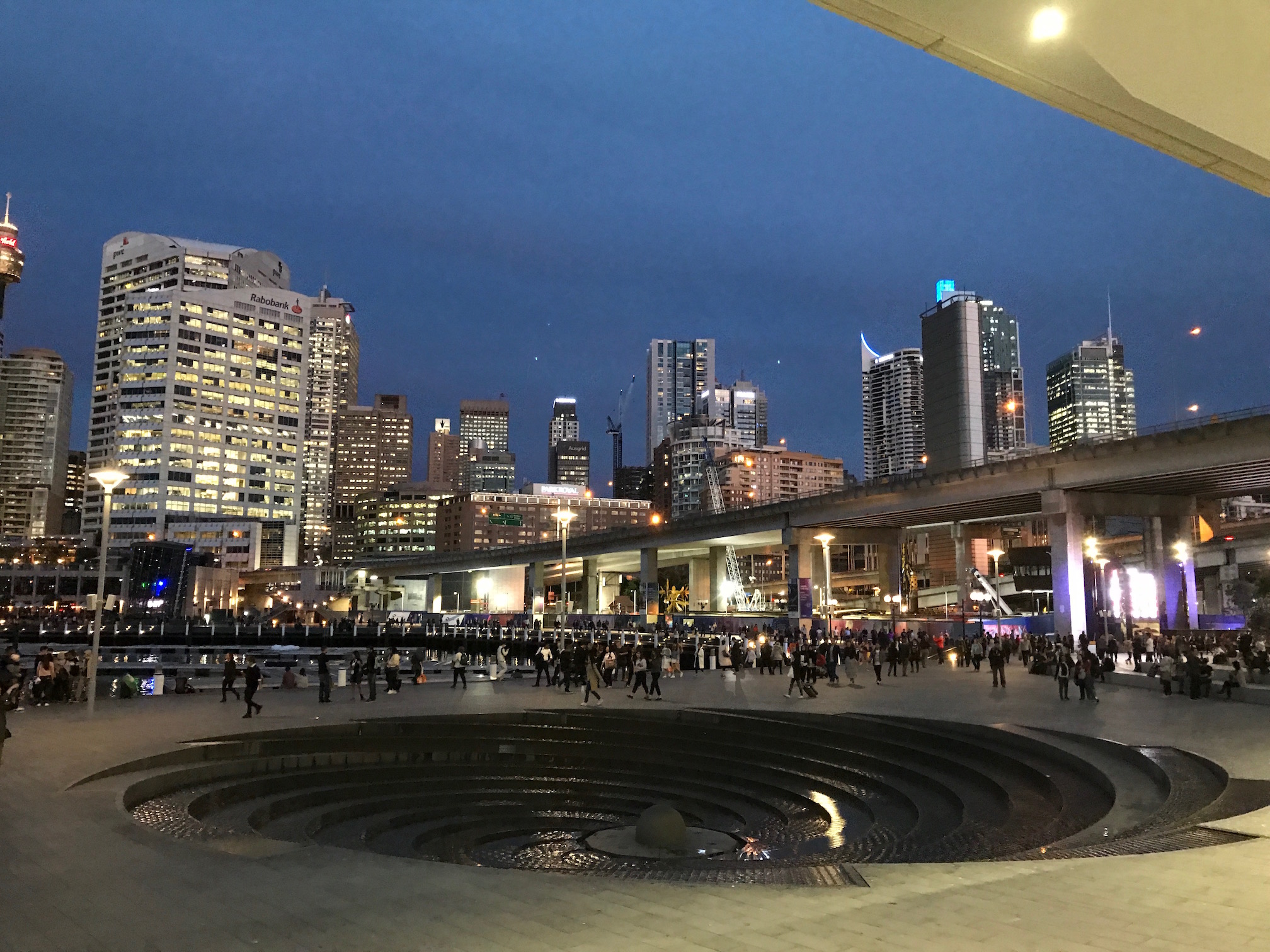A view of the harbor.

Another view of the harbor.

Yeah. Someday, I’ll be back.

For the fourth day of UAI 2017 (August 14), I skipped my 4:30am workout to get two more full practice runs of my talk. Thus, by the time I entered the conference venue, I was feeling confident.

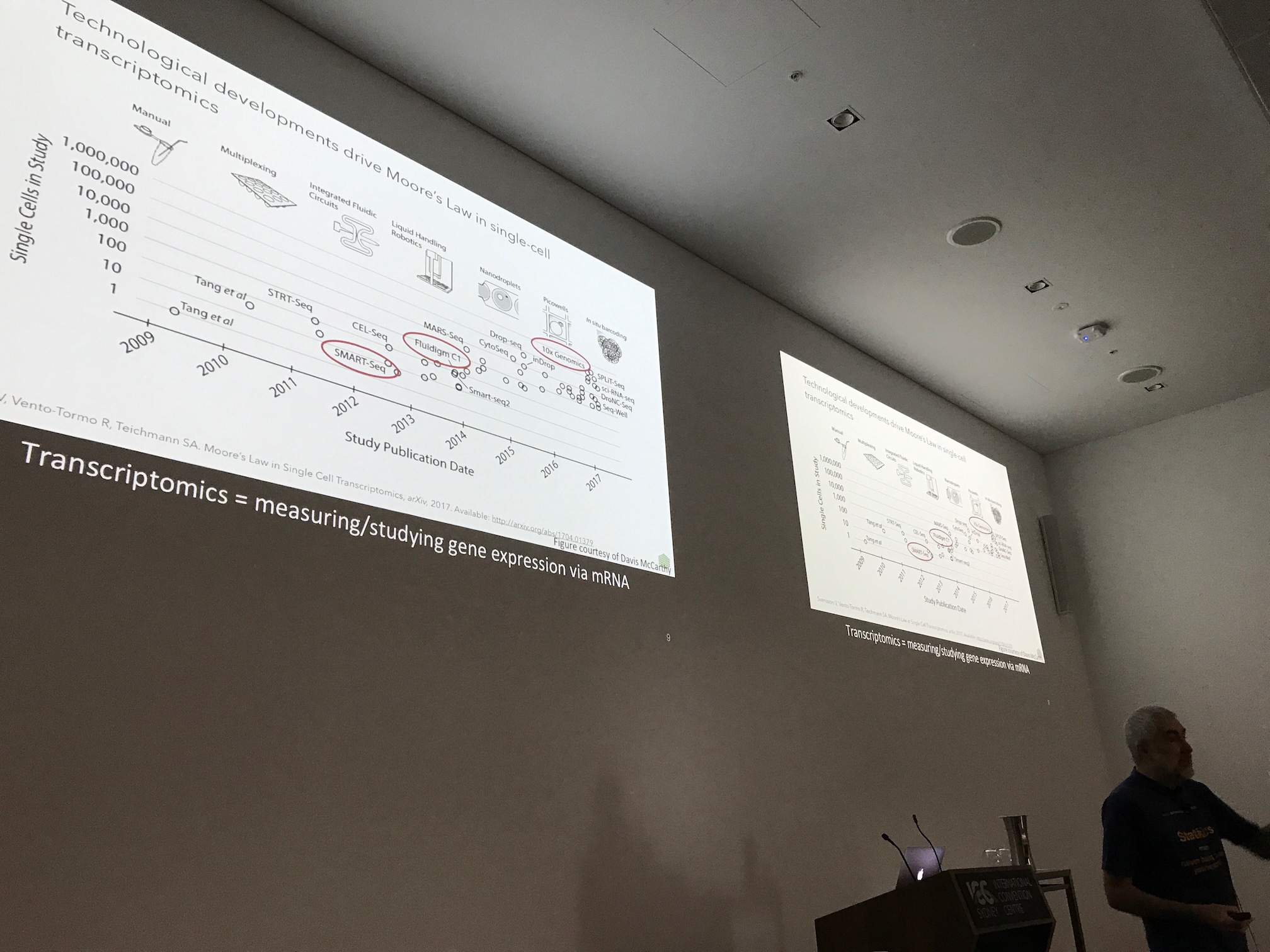Professor Terry Speed gives the keynote talk of the day, and the fifth one overall for the conference.

The day started off with our last keynote for the conference, presented by Professor Terry Speed who currently works at the Walter and Eliza Hall Institute of Medical Research in Australia. Interestingly enough, he used to be a Berkeley statistics professor until his retirement in 2009.

His talk reminded me of Professor Heller’s talk from the other day. There’s a lot of work being done at the intersection of medicine and artificial intelligence. My impression is that Professor Speed’s work is more about RNA and DNA sequencing, while Professor Heller’s is about modeling diseases and health conditions. There might be overlap with the techniques they use, since both briefly mentioned (recurrent) neural networks. Yeah, they’ve fallen for the hype.

While Professor Speed is funny and skilled at presenting, I had a hard time processing the technical content, because I kept mentally rehearsing for my talk. This also happened during the first oral session (on causality) which preceded the one that contained my talk. Does anyone else find it hard to focus on talks that precede theirs?

Finally, at around noon, after several Disney Research people taught us about stochastic gradient descent for imbalanced data, it was my turn.

Whew … I walked up and got my laptop and clicker set up, though before I could begin, the conference chair gave a few remarks about my paper and then presented me with the Honorable Mention for Best Student Paper Award. After some applause, I also pointed out my coauthor John Canny in the audience, and got everyone to applaud for him as well. Then I began my talk.

I’m pleased to report that my talk went as well as I could have hoped for, with one exception that I’ll bring up later.

Here’s the list of rather sloppy reminders that I made for myself and which I reviewed beforehand:

• Don’t be flat-footed, don’t stand like a robot.
• Don’t swing side to side!!
• Must stay vigilant and alert!
• Must not have a flat voice. Try to vary it. Lots of deliberate pauses. With smiles!
• Talk LOUD, since I will likely be moving away from the microphone.
• Don’t put my hand in my pockets!
• Thank them at the beginning for the award, and at the end thank the audience for their attention.

I also wrote talk-specific reminders to include phrases such as “I hope you remember this” when reaching this slide, and so forth.

One thing that’s perhaps unique about me is my stance on giving talks. I touched up on this briefly when discussing my class review for Algorithmic Human-Robot Interaction, but I’ll expand the discussion here with some bold text to catch your attention.

I view talking in front of a large audience as an absolute privilege that I CANNOT waste. Thus, my talk must be polished, but in addition, I must make it MEMORABLE and keep the viewers as ALERT as possible. This means I need to be loud, funny, and highly active. Even if this comes at the cost of a slight reduction in the amount of technical material that appears on my slides.

For the vast majority of conference talks, while some audience members pay rigid attention, many will also be checking their phones and laptops. Realistically, there’s no way to keep everyone’s attention for the entire talk, especially in conferences when there are many talks back-to-back. Even with coffee, people can’t absorb all this information. Thus, I think it’s best to simply get the audience interested so that they can look up the material later in their own time.

One absolute sure-fire way to lose the already-fragile attention span of humans is to stand frozen behind a microphone and read off text-filled slides (or a pre-made script) with a flat voice. Sorry, but when people do that, I want to yell at them: What are you doing?!? You’re wasting such a great opportunity to impress your audience!! The fact that the majority of conference speakers — mostly students, but sometimes faculty are guilty of this as well — still do this is simply mind-boggling to me. It’s completely baffling.

I understand that non-native English speakers might have difficulty with knowing what phrases to emphasize and so forth. But that doesn’t mean they can’t smile and be active when presenting, and the people who are guilty of robotic speaking are not always non-native English speakers.

Of course, there are certain times when it’s best not to follow my speaking techniques. I would obviously not apply this style at a funeral. Academia, however, is not entirely conservative in presentation style. Sure, you can be a boring robot reading off a script, but you can also be active and constantly be in engagement with the audience and no one’s going to stop you.

Whew. Anyway, sorry for that mini-rant but this felt like something important I should bring up. You can expect that whenever I give a polished academic talk at a conference, I am not going to be a boring or typical speaker.

For my talk, I did not stand behind the lectern with the microphone; I stood in front of it like Terry Speed did (see the picture above).

I also deliberately did not walk too fast when talking. The key is to walk a little bit, stand still, point the laser pointer at the slides, make a joke or two, make eye contact with the audience, and then slowly walk to the other side of the room.

I think the talk was great. I followed my advice and made some comments to get the crowd to laugh. One of them, for instance, was “please remember this figure for the rest of your life.”

OK, now what was that one “exception” I referred to earlier? It happened during the question-answer session. Professor John Duchi asked if I could prove that the method “converges to the correct posterior distribution” or something like that. I must have laid an egg because I don’t think my answer satisfied him (though to be fair, I thought his question was too vague).

Then John Duchi and coauthor John Canny (who were sitting next to each other) started discussing amongst themselves, as humorously pointed out by conference chair Kristian Kersting. Incidentally, Kristian was standing next to me during this Q&A to repeat questions from the audience, since I can’t hear/understand them. He had to relay John Duchi’s question to me even though John was literally five meters away from me.

After my talk concluded, the other conference chair, Gal Elidan, came to me and shook my hand (I didn’t see him do that to anyone else). Throughout the rest of the day, no less than six people came to me and said they liked my talk.

I certainly felt relieved after presenting. It was also our lunch break. I wasn’t sure what to do, but fortunately, John Canny came to my rescue and said that I should join him plus a few others for lunch. It turns out those “others” were: Gal Elidan, Kristian Kersting, Terry Speed, and John Duchi. Gulp. I would of course never have the courage to ask to join them for lunch myself, given that just about the only thing I’m better at than those guys is blogging.

John Duchi made the choice to eat at a small lunch/bar place called Social. I ate a pork burger and mostly watched the conversation, since I was unable to get involved.

We finish lunch at Social. From left to right, we have Professors Terry Speed, Kristian Kersting (behind Terry Speed), Gal Elidan (behind John Duchi), John Duchi, and John Canny.

After that, we had another oral session and then a poster session.

The third day of UAI 2017 (August 13) started off with Stanford Professor Christopher Ré giving the first keynote talk of the day about his group’s project called Snorkel. Chris is epitome of a “rock-star academic,” and he has a ridiculous amount of publications in the last few years. His lengthy list of awards includes the well-known MacArthur “Genius” Fellowship.

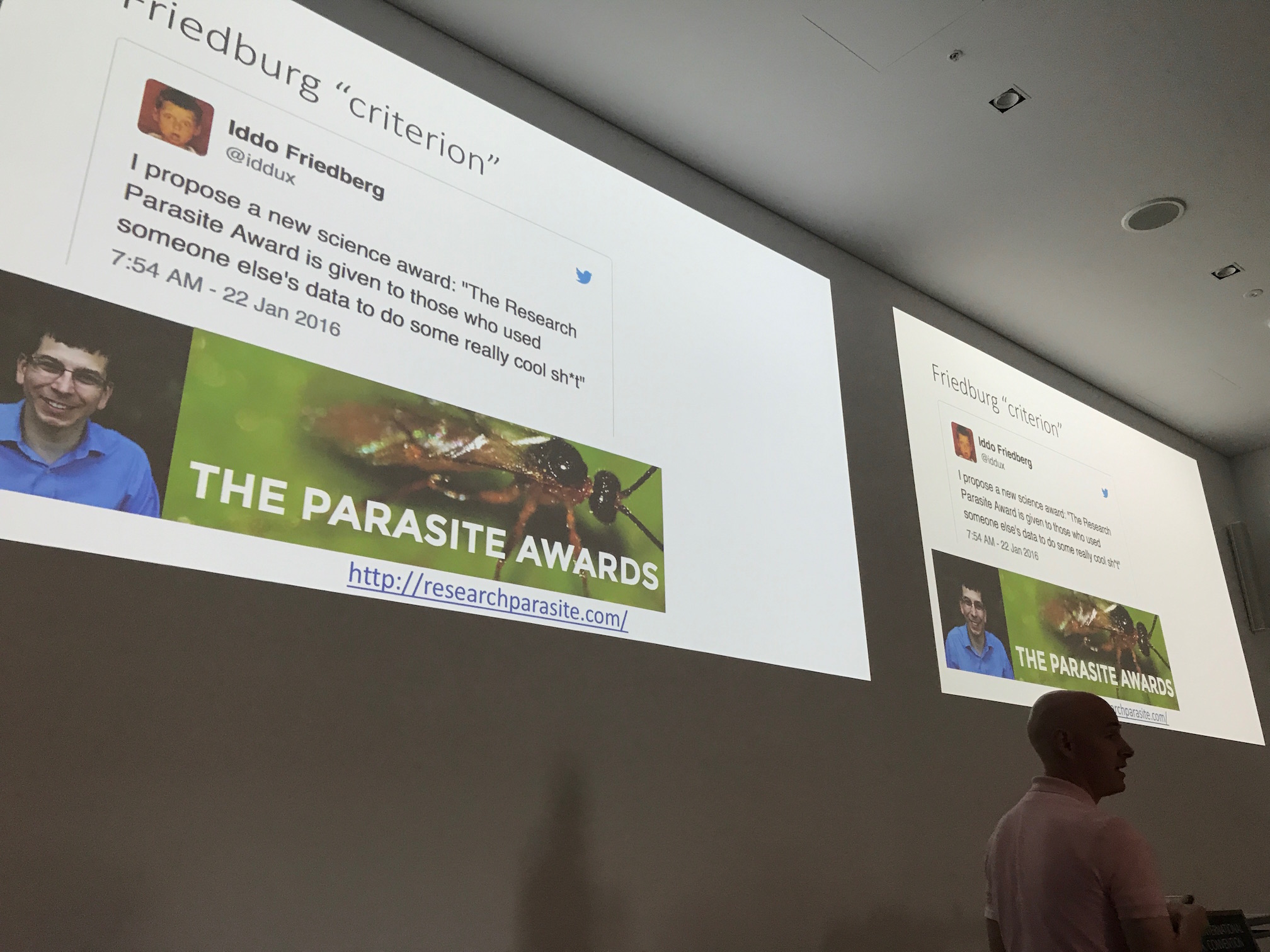Stanford Professor Christopher Ré gives the first keynote talk of the day.

I really enjoyed Professor Ré’s talk, both for the content and for the “style” (i.e. at the right technical level, good visuals, etc.). He inserted some humor now and then, as you can see in the slide above. Anyone want to win the parasite award? Heh. I also try to include humor in my talks.

Anyway, as I mentioned earlier, the main technical part of the talk was about Snorkel. It’s an important project, because it helps us deal with “dark” or unlabeled data, which is what the vast majority of data will look like in real life. How can we make sense of dark data, and “clean it up” to make it more useful? This is critical because, as Professor Ré said in the talk:

Training data is the new, new oil.

(Yes, he said “new” twice.)

I was amusingly reminded of Andrew Ng’s famous (or infamous, depending on your opinion) phrase:

AI is the new electricity.

In case you are curious, I agree with both of the above quotes.

You can find more information about Snorkel on the project website. What’s great is that there are also lots of blog posts. His group really likes to write blog posts! At least I have something in common with them.

The first oral session was about “Representations”, a research sub-field which I am unfortunately not familiar with, and so I had an extremely hard time following the material. I tried to gather pieces of what I could and recorded anything interesting in my ongoing Google Doc containing my notes from UAI 2017. As I stated in my last blog post, I do not try to follow talks in their entirety — I couldn’t do that even if I wanted to — but I record bits and pieces of intriguing stuff which are candidates for future investigation.

During breaks, I worked on outlining these blog posts; I drafted them in Google Docs.

The second oral session was about … reinforcement learning! Awesome. At least I should have more background information for this material. Of the four papers presented, the fourth one seemed to have the most interesting material in it. The UAI organizers must have agreed, because the authors (Shayan Doroudi along with Philip Thomas and Emma Brunskill) won the UAI 2017 Best Paper Award for the paper “Importance Sampling for Fair Policy Selection.”

Fairness is becoming a recurring theme in research and academia nowadays along with safety and (as you’ll see later) health care. The talk was excellent since Shayan has good speaking skills. He motivated the problem with a quick example of choosing between two policies, one of which was obviously better than the other. Despite the apparent simplicity of choosing the policies, importance sampling approaches can actually choose the worse policy more often than not.

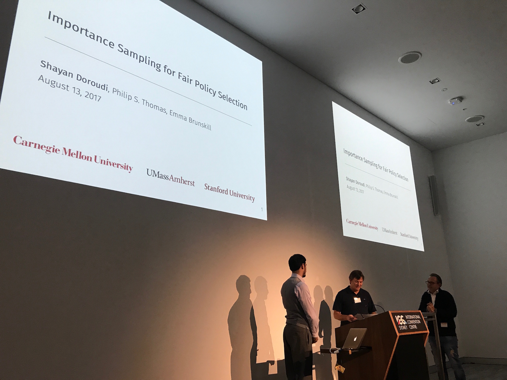Shayan Doroudi (to the left) being presented with the UAI 2017 Best Paper Award by the conference chairs. Congratulations!

We now have the following award-winning reinforcement learning papers:

• Importance Sampling for Fair Policy Selection (UAI 2017 best paper)
• Modular Multitask Reinforcement Learning with Policy Sketches (ICML 2017 runner-up best paper)
• Value Iteration Networks (NIPS 2016 best paper)
• Dueling Network Architectures for Deep Reinforcement Learning (ICML 2016 best paper)

At some point, I’d like to grind through the details in these papers. I know the high level idea of each of these but aside from perhaps the dueling networks paper, the details elude me.

After a brief lunch break with another student from India — whom I found standing alone and thus it made sense for us to go to lunch together — we had our second keynote talk. Duke Professor Katherine Heller gave a talk about machine learning in health care. Gee, is anyone seeing a trend with machine learning applications?

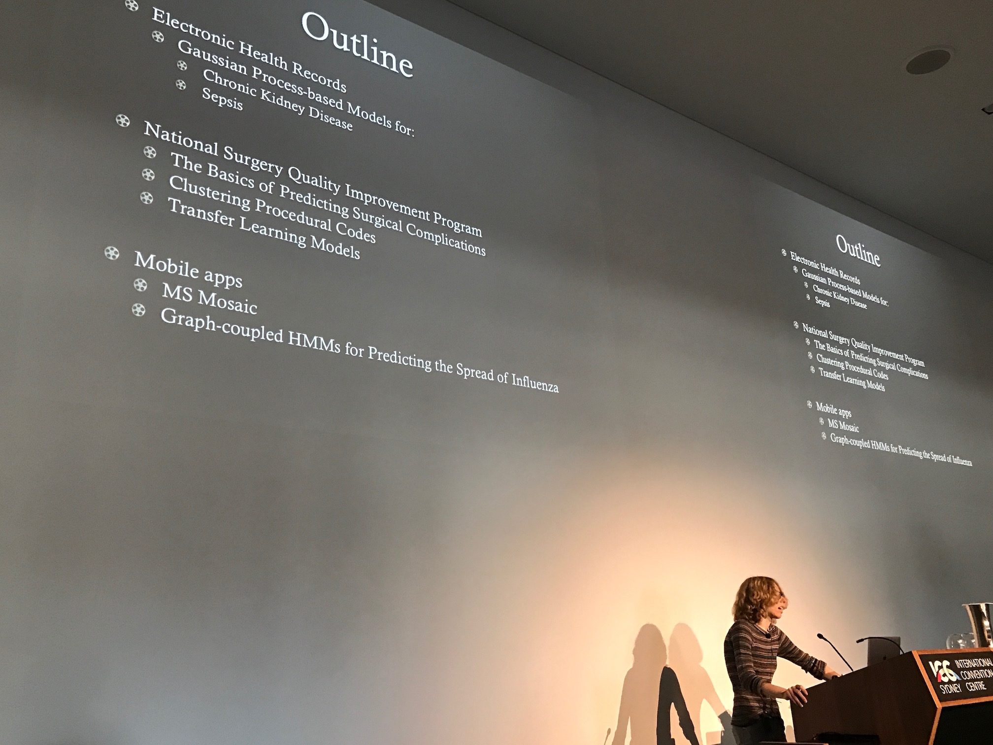Katherine Heller gives the second keynote talk of the day.

You can see the outline of her talk in my picture above. I remember that she discussed the following topics:

• Health conditions: chronic kidney disease, sepsis, and multiple sclerosis.
• Health issues: delayed diagnosis results in problems, surgery can introduce complications; her exact figure was 15% of the time but there are obvious simplifications with numbers like that.
• Modeling health issues: using graphical models with latent variables. Basically, given health conditions (or a sequence of conditions measured at times) what can we say about the patient’s health? I also saw a few mentions of RNNs and LSTMs there (wow, really?) and would be interested in learning more.

Given that much of the talk was about, I believe, modeling health care, I sometimes wonder how accurate our models are. The United States has one of the most inefficient health care systems in the developed world, and I wish we could use some machine learning to cut away at the inefficiency.

After Professor Heller’s talk, we had the usual poster session. I managed to engage in a few interesting one-on-one conversations, which is good enough for me!

We then had a special event provided by the conference: a dinner cruise along Darling Harbor. Awesome! The buffet options included a wide range of food options: prawns, Indian chicken curry, Thai fish curry, pastas, potatoes, and of course, lots of salad options.

UAI 2017 conference attendees lining up to get dinner.

I don’t know about how others feel, but every time there’s an event like this where I have to pick my own seat amidst a large dinner gathering, I worry and overthink it way too much. Fortunately, there was a student who I met earlier at the conference who told me to sit near the center (gulp) of a table filled with other graduate students, thus saving me the stress of coming up with the decision myself. I was happy with this because it meant I wasn’t sitting by myself, and because it’s better for me to know other graduate students (and potential future collaborators/colleagues) rather than, for instance, industry sponsors.

Yes, it was extremely noisy in the ship, and I couldn’t participate in substantive conversations, but hey, at least I was sitting with other graduate students. And it seemed like there was some ongoing discussion regarding my blog, judging by how several of the other students nearby kept looking at my name tag in order to correctly spell my name in Google.

Throughout the cruise, we would frequently walk to the top of the ship and view Darling Harbor.

A view of Luna Park.

A view of the Sydney Opera House.

For the second day of UAI 2017 (August 12)¹, I followed the same initial routine from the previous day. I woke up early, had a 4:30am gym session, ate a hearty breakfast at the hotel’s buffet, and then walked over to the conference venue. The talks were held in the room shown in the following image:

Room C4.8 in the ICC Sydney building.

Yeah, it’s a fairly small room. Compare that to the room used for the ICML keynote talks, which is in the same building. Wow!

Fortunately, the second day of UAI started off better than the first one, since the captioner (a.k.a. “CART provider” or “stenographer”) arrived. Whew.

At around 8:30am, the day began with some opening remarks from one of the chairs. After that, it was time for MIT robotics professor Leslie Kaelbling’s one-hour keynote talk on Intelligent Robots in an Uncertain World. It was a nice, relatively high-level talk which centered on Partially Observable Markov Decision Processes (POMDPs) and belief states, with applications that focused on robotics.

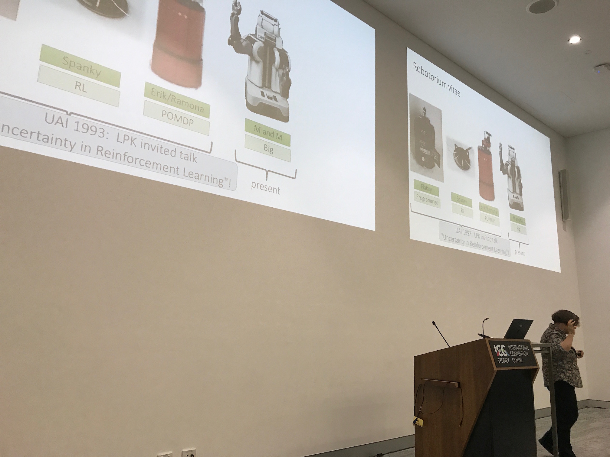Professor Kaelbling gives the initial keynote talk for UAI 2017.

The experiments that she showed in the slides involved the PR2 robot, which I assume is one of the primary robots in her lab. I wish I could use the PR2 one of these days, or at least a robot similar to it.

The final part of her talk contained a request for the UAI community to figure out how to perform action selection in belief spaces. In other words, if we don’t know everything about the environment (which is always the case in real applications) we have to pick actions on the basis of what we believe about the world.

Overall, it was an excellent talk. There were a few sections that were relatively difficult for me to follow, but I’m not sure if it was because there was too much information to process in the slides (some of them had a lot!) or if it was because I had a hard time getting used to the captioning.

After the keynote talk, we had oral sessions. In these, authors of papers accepted to the conference give 20 minute talks. Not all the papers have oral talks, though; they’re reserved for those with the highest reviews. Also, typically the first author is the one who gives presentations.

Today, there were four oral sessions, each of which consisted of one broad research topic and three research papers in each (so each session was an hour long). The first oral session was about deep models. Yay! Ming Jin started off the oral sessions with his excellent talk on inverse reinforcement learning.

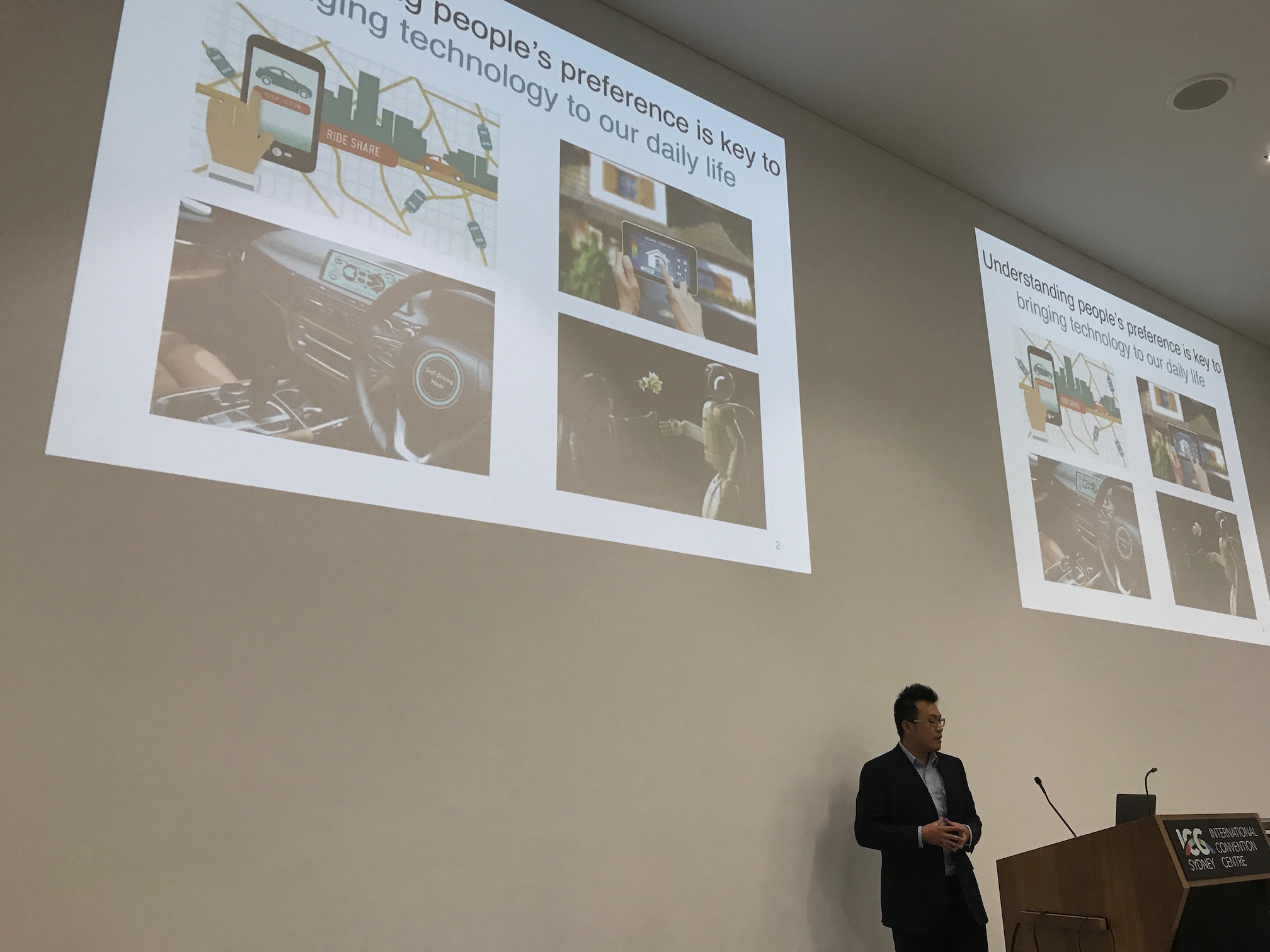UC Berkeley electrical engineering PhD student Ming Jin gives a talk about his paper Inverse Reinforcement Learning via Deep Gaussian Process.

The two other talks for this oral session were also interesting and perhaps more related to core Deep Learning research.

The second oral session was on the subject of machine learning, which is probably not the best name for it, but whatever. Unfortunately, the papers were quite mathematical and the speakers were a little difficult to understand (the captioner had major difficulty) so it was hard for me to get much out of the talks beyond trying to extract every ounce of information from the slides that I could.

After a break for lunch — though I was simply too full from eating earlier and had to pass — we had our second keynote of the day, Expectations in Learning and Inference by Professor Amir Globerson of Tel Aviv University.

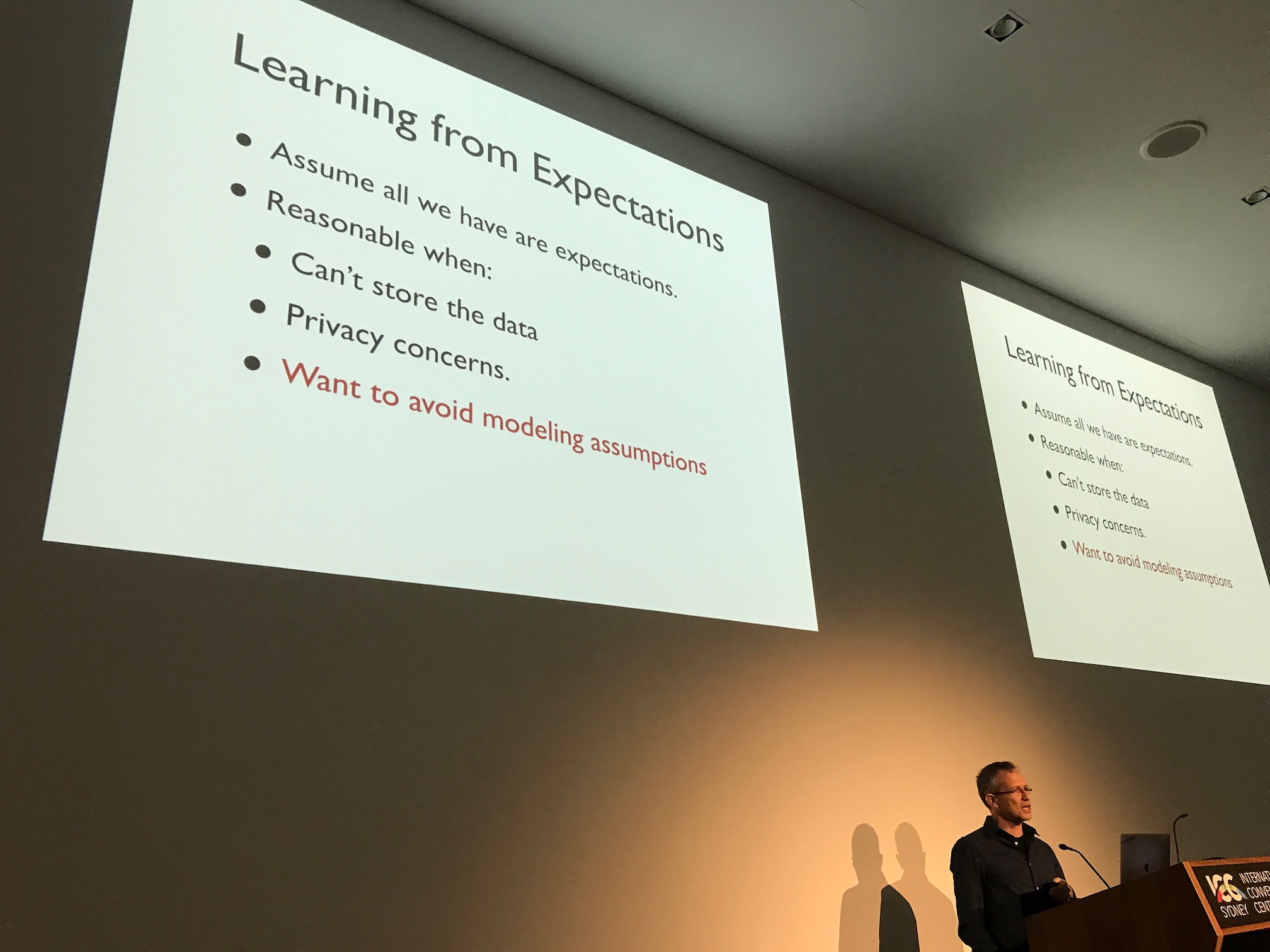The second keynote talk of the day.

This talk was more about math, in particular about expectations and probabilities. What happens when we aren’t given data but are given the expected value? What can we determine from it? (See the slide above for the related context.) The technical contribution was probably the development of bounds for not probabilities, but the minimum of probabilities over a certain class (if that makes sense?). I unfortunately had a harder time understanding this talk compared to the first keynote. I thought I could follow slide by slide and sentence by sentence in the captions when I saw the transcripts, but I couldn’t piece together a good story. Maybe this has happened to other people?

In any case, for me I long ago decided that for research talks, I don’t try to understand everything but instead, I find any interesting points and then follow-up on these later, either by emailing the author or (more likely) simply searching online. Google has been great for people like me.

We had two more oral presentations after this second keynote. In between the two, I had an entertaining conversation with another student from the University of Helsinski who told me that hearing aids should have some way of blocking out background noise. I told him that, sadly, they’re already supposed to do that, though he didn’t give up and said that we should use machine learning to make them block out noise. Yeah, that would be great.

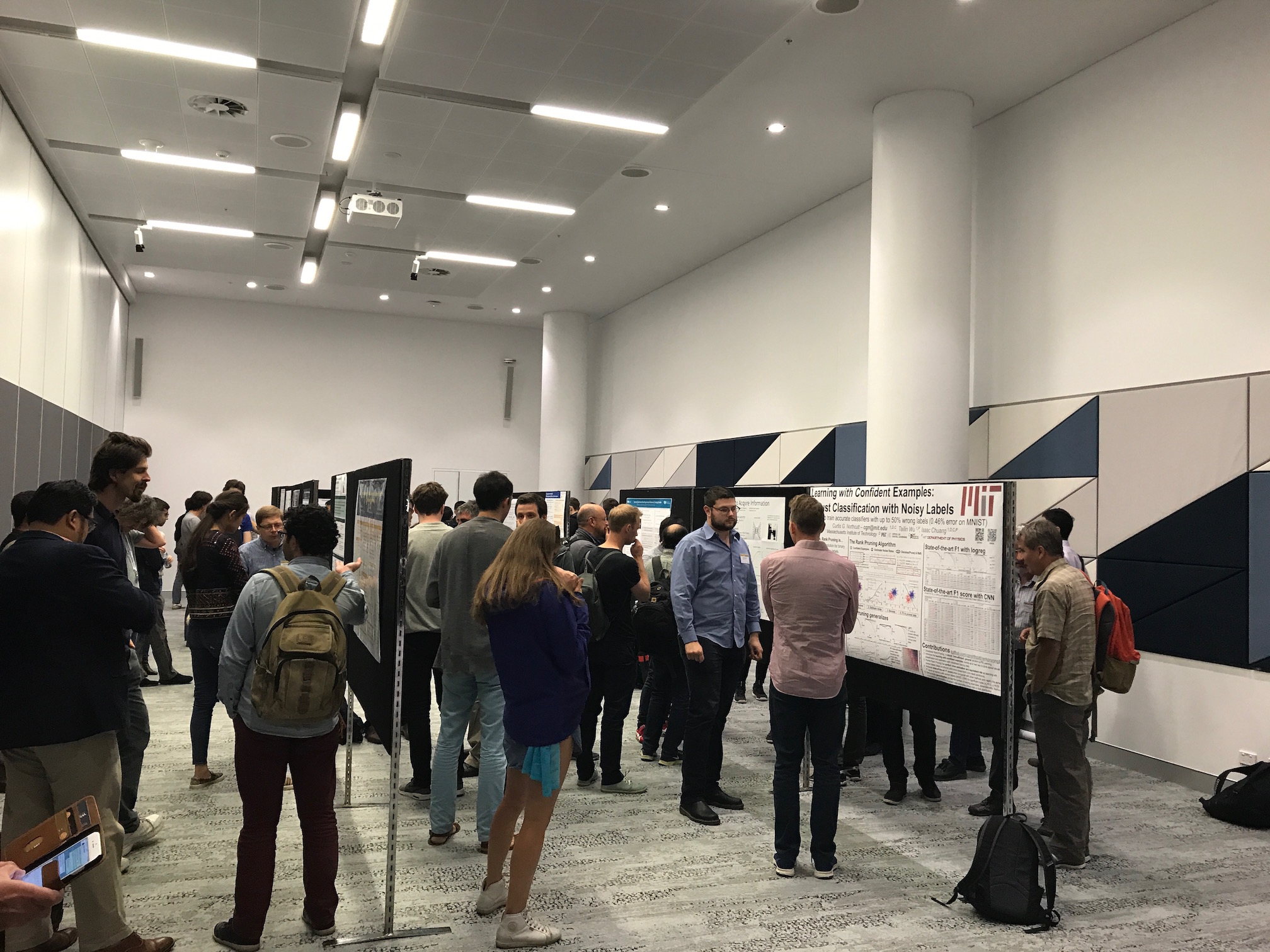The poster session for today.

We wrapped up the day with a poster session which featured roughly one-third of the UAI 2017 papers. (There are also poster sessions in day three and day four of the conference.)

After this, I went to the nearby mall and found a quick, cheap Middle Eastern restaurant for dinner. I ate by myself as I didn’t know anyone else, and I couldn’t find any lonely person who I could pounce on with an invitation, but that was OK with me. I just wanted to see what the city had to offer, and I’m pleased to say that I was not disappointed. Darling Harbor has a ridiculous ton of awesome restaurants. It’s food paradise for someone like me.

The view of the lovely harbor at night. The conference is in the large building located at the center-left with the lights on. To its right is a giant mall (which the photo doesn't entirely reveal) with a LOT of stores and restaurants. Wow.

---

Sadly, the day did not start out well. When I opened my inbox this morning (August 11), I saw this from the transcription agency which was supposed to (spoiler alert!) provide captioning services:

Hi Daniel,

Thank you for the confirmation. As at 9:00pm yesterday we were still awaiting confirmation of the details and were not sure that the stenographer was still required for today. As such, it is unlikely that [name redacted] will make it to the venue today. I have spoken with her this morning and she will be there ready to go on Tuesday morning.

I have passed on the information below and [name redacted] has your phone no.

I am very sorry that we are not able to cover the captions for today. It has been difficult, with the lack of communication this week, to know what was happening.

Good luck with today.

Ouch. Where to begin?

I had carefully arranged for captioning services to be arranged for this conference. I looked at my email records. On June 15 I sent an email to Berkeley’s DSP, and received acknowledgement from them that same day, that we should arrange for accommodation services (either captioning or sign language interpreting). The conference, as you know, starts August 11. That’s almost two months. And the paper got accepted on June 12 so I couldn’t have known I would be attending UAI before June 12.

A month later, on July 15, I had sent (and again, received acknowledgment from them) the day and times of the talks, which included August 11. I’m not sure if the exact rooms had been set up, but at least the times were known. And of course, we all knew that UAI was in the ICC Sydney building. Once again, I couldn’t send this email earlier since the schedule was not available on the conference website until then.

Thus, on July 15, I thought that the captioning services were essentially set up. Indeed, after I had repeatedly questioned Berkeley’s DSP, they sent me this email on August 3 which implied that things were OK:

Moving forward. The CART provider(s?) are booked, and I’ve passed the schedule updates along.

I’ll put you in touch with them before the end of the week to discuss details and logistics, as well as prep materials if possible.

Yet on August 11, the day the conference began … I got that email above. Gee, doesn’t that directly contradict the August 3 email from Berkeley’s DSP? I double checked, and the schedule I sent to them on or before that day definitely included August 11, not to mention that I explicitly included August 11 in the written portion of the email (and not in an attachment).

I was also intrigued by the fact that the transcription agency emailed me directly about this, but didn’t do so until late at night on August 10 (and I had gone to sleep early due to jetlag). Why didn’t they email me so sooner? It’s also not like my contact information is completely invisible; a simple Google search of my name (even if it’s from Australia) should have this blog as the #1 hit. Moreover, I saw an email thread between Berkeley’s DSP and the transcription agency that went back a few days which was forwarded to me on the morning of August 11. It appears that the transcription agency was aware of my email on or before August 9 (to be fair, I’m not sure the time zone). Somewhere, there must have been some massive mis-communication.

Yeah. I got completely blindsided.

I think back to my previous grievances with accommodations: see here for my prelims and here for the BAIR retreat. One thing that would especially help in these cases is if I could directly contact the agencies providing those accommodations.

After I return to Berkeley, I am going to talk to DSP and demand that for future conferences, I am able to contact whatever captioning (or sign language interpreting) agency they use. I will always copy Berkeley’s DSP to these emails, and DSP is certainly free to email and/or talk to them so long as they always copy me in emails and give me the details of any phone conversation. Always.

If they refuse, then I will figure out how to sue DSP.

In addition, I will switch to figuring out how to get an automated captioning system set up on my laptop for future conferences as I have lost interest in the hassle of setting up accommodations.

In a foul mood, I trudged over to the room of the talk (see picture below) and hoped for the best.

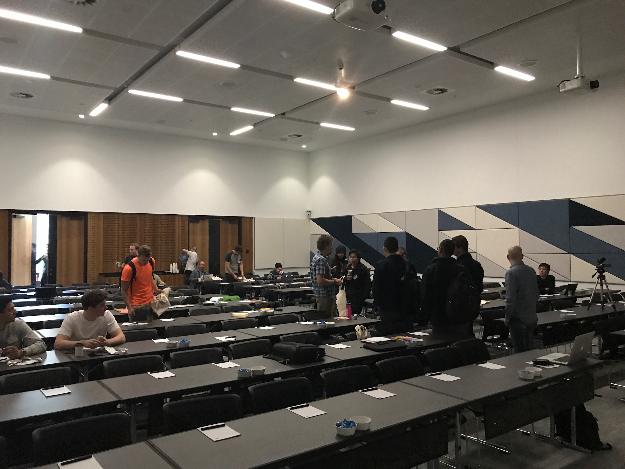The room where the tutorials were located. This was actually taken after the first tutorial, but I decided to put this picture first in the blog post because ... artistic license.

Tutorial 1 of 4

Fortunately, my mood soon brightened once the first talk began at around 8:45am, featuring Assistant Professor John Duchi of Stanord University. He’s known as a machine learning rockstar. I’ve always wondered how he is able to produce so much mathematical research and have time for pursuing other physical activities such as running and participating in triathlons. (When I was applying to graduate school, he told me he was considering accepting the University of Washington’s faculty position, and I sheepishly thought that I could be one of his students there.) I knew I was in for some great content, and on the plus side, his voice is relatively easy to understand. I took a lot of notes (in Google Docs) of his talk. It was divided into two parts: convex optimization and non-convex optimization. Yeah, not the most creative division, but it’s the content that matters.

He started by providing some basic definitions of convex optimization and so forth. Given my background in EE 227BT and EE 227C in Berkeley, I was fortunately aware of this material. Nonetheless, I was happy he went over the concepts slowly. He introduced us to the style of convergence proofs that people use in his sub-field, which often involves relating expressions of the form \(\|x_{k+1}-x^\star\|_2\) and \(\|x_k-x^\star\|_2\).

John then moved on to discuss interesting topics ranging from AdaGrad — which is probably his most well-known research contribution — and about how to transform non-convex problems into convex problems, which is a technical way of saying “let’s make the hard problems easy.” Along the way, he inserted some humor here and there. For instance, when talking about the slide in the following image, John referred to the function as “Batman”:

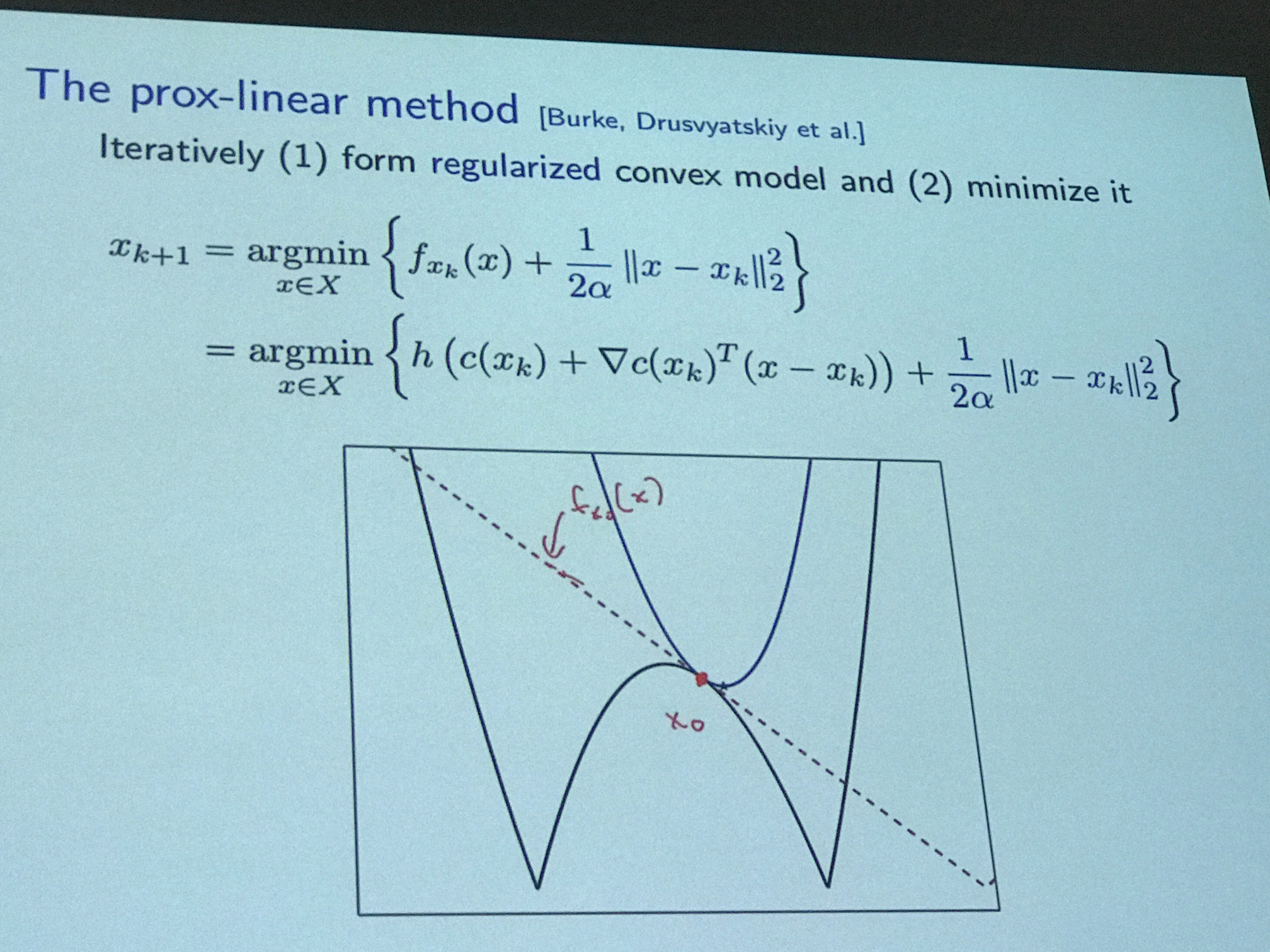The "Batman function", according to John Duchi.

Because, hey, doesn’t that look like Batman, he asked rhetorically. John then said he was watching too much Batman. I must have misheard because I don’t believe that one iota.

There were a lot of references to go through in the last few slides. I hope to skim a few of them to get a feel for the work, but unfortunately John hasn’t posted the slides online anywhere. But I remember that a lot of them were his own papers anyway.

Tutorial 2 of 4

After a quick coffee break (thanks but no thanks, that lovely cappuccino from the hotel’s buffet was more than enough to keep me awake), the second speaker, Arthur Gretton, gave his talk on comparing probability distributions. The main idea: given samples from two distributions \(P\) and \(Q\), do the two distributions differ? In addition, what can we learn about these distributions, and can we figure out their dependency relationship? Many interesting questions arise out of this, and anyone who has been following machine learning seriously should know that problem of trying to distinguish between samples from two probability distributions is precisely what the Discriminator tries to do in Generative Adversarial Networks.

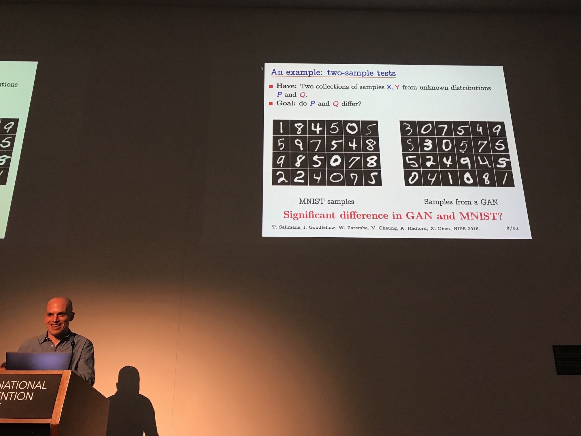Anything GAN-related is going to catch my attention!

Indeed, Gretton discussed GANs for a few slides, and in fact I think he may have talked more about GANs than Shakir and Danilo did in their Deep Generative Models tutorial later in the afternoon. However, GANs weren’t the entirety of the talk. Much of it was dedicated to some of the technical details regarding “Maximum Mean Discrepancy” and other metrics for comparing distributions.

Unfortunately, I couldn’t really follow the talk. Aside from the stuff on GANs, and even not entirely that — I don’t know how Wasserstein GANs work, for instance — I barely understood what was going on at the technical level. Yes, I know the talk is about distinguishing between two distributions, and yes that’s obviously useful. I just didn’t get the technical gist of the talk.

On top of it all, I could not understand the speaker’s voice despite sitting in literally the seat which was located closest to where he was talking.

Tutorial 3 of 4

The third talk was the one I was most excited about: Deep Generative Models, presented by Shakir Mohamed (blog) and Danilo Rezende (blog), both of whom are research scientists at Google DeepMind, and both of whom have excellent blogs. I hope that mine will soon be as useful to machine learning researchers as theirs are!

The speakers do some last-minute discussion before giving their joint. Gal Elidan (to the right) is one of the conference organizers.

Danilo took over the first half of the talk and gave a long, borderline overkill motivation for why we like generative models, but I liked the examples and it’s important to try and sell one’s research. For the more technical part of the talk, he discussed fully observed and latent variable generative models, and frequently compared different sub-approaches with pros and cons of each. Unfortunately I wasn’t too familiar with many of these models, and I couldn’t understand his voice, so I didn’t get much out of this.

I benefited more from Shakir’s half of the talk since he was relatively easier for me to understand. (By the way, I have to reiterate that when I talk about not understanding speakers, it’s emphatically not a criticism of them but simply a limitation of what I can understand given my hearing limitations.) Shakir was extremely engaged and talked about the score function estimator and the reparameterization trick, both of which are featured on his blog and which I had previously read beforehand. It was also nice for Shakir to discuss all the ways in which people name these; I learned that Radon-Nikodym derivatives are another way of referring to the policy gradient used in REINFORCE (i.e. Vanilla Policy Gradients).

I certainly think I learned more about the big picture of deep generative models after Shakir’s half, so the talk was on the whole positive for me.

Tutorial 4 of 4

The fourth and last tutorial for the day was about Machine Learning in Healthcare. In general, health care-related talks don’t have much to do with the majority of UAI papers, but the plus side is that they’re much more readily applicable to the real world. And, y’know, that’s important!!

Unfortunately, due to visa issues, Suchi Saria (the speaker) couldn’t attend the tutorial. Thus, her talk was pre-recorded and provided as a video. I stuck around for the first few slides, but unfortunatey, I couldn’t understand what she was saying. It would have been hard enough to understand her in person, but having it via video made it even worse. The slides were informative, but the material isn’t related to my research. Thus, I quietly left the talk after the first few slides, took a seat with a nice view of Darling Harbour, and got to work on my blog.

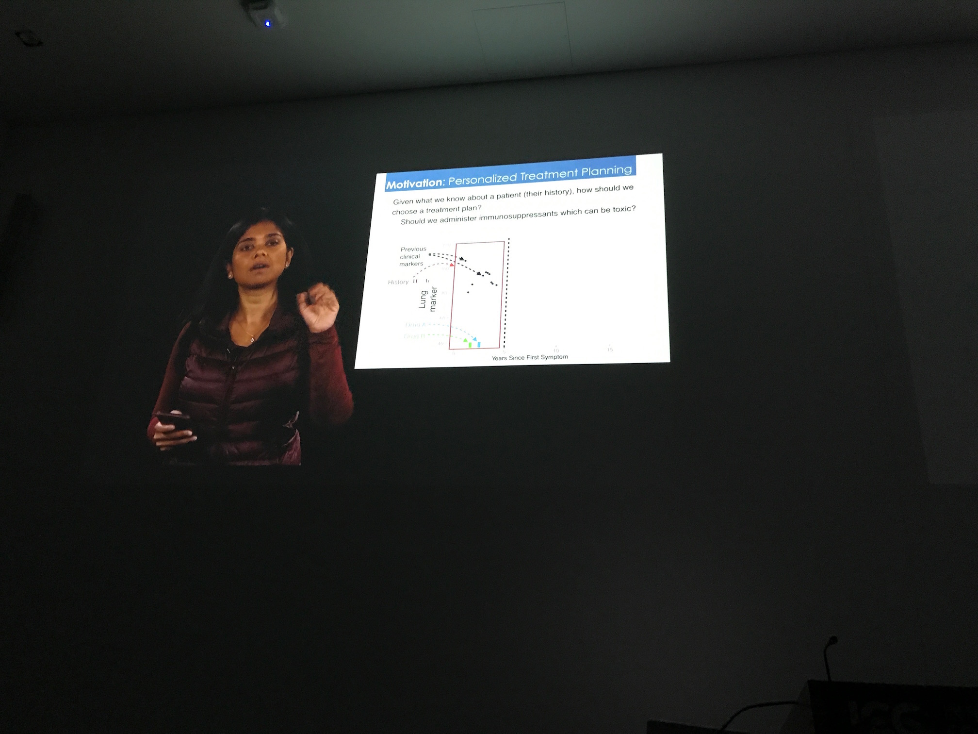The fourth speaker couldn't attend due to visa issues, so her talk was pre-recorded.

But in all fairness, put yourself in my shoes. I think if you were someone who could not understand what a speaker was saying and had the choice between sitting for an hour to listen to a pre-recorded talk that wasn’t in your area of research, I think you would do the same.

On the morning of August 10 (a.k.a. my birthday), I arrived in Sydney, Australia. It’s my first time in Australia. I am attending the Thirty Third Conference on Uncertainty in Artificial Intelligence (UAI). UAI is probably known in AI circles as the little brother of the ICML and NIPS behemoths, but it’s still a top-tier academic conference. I would say ICML and NIPS are the clear-cut top two conferences in AI, with UAI being “1b” to them.

The reason why I’m attending is that I am presenting a research paper, An Efficient Minibatch Acceptance Test for Metropolis Hastings, which was accepted there. I feel very fortunate to also receive the Honorable Mention for Best Student Paper award. (There are three awards given by this conference: one for the best paper, one for the best student paper, and one honorable mention for the best student paper.) I’ll be giving a talk on the fourth day, so until then I’ll just listen as much as I can.

The lovely view of Darling Harbour from my hotel room. UAI (also ICML before that) is held in the building to the top center with the white cover on it. Sorry for the picture quality; you can tell it was taken through a window.

I got to the hotel sufficiently early on August 10 to relax for a bit, and you can see the excellent view above.

Though to be honest, I was a bit anxious and didn’t fully relax. August 10 was also the next-to-last day of ICML, and I was looking at Twitter to see all the tweets with the #icml2017 hashtag.

And … wow, ICML is crowded! Now, UAI isn’t going to be as crowded, but there will still be lots of people. This raises some serious concerns for me, in particular (a) how to find someone to talk to, given that in large groups, others are able to quickly find conversationalists while I resort to watching people talk, and (b) if I did find someone to talk to, how would I understand that person?

I didn’t come up with an immediate solution to this. On the other hand, I resolved to do something for the conference that I don’t ordinarily do, but which I should be doing more often:

I will never let someone — who is talking to me — get away with saying something that I don’t understand. I will ask that person to repeat what he or she says as many times as needed.

Is that clear? For instance, if I’m talking with another person about research and he says something which I can somewhat tell isn’t that important to understanding the gist of our conversation, I don’t care. I am asking him to repeat.

I’ve gotten reasonably skilled at telling what parts are or are not important to understanding the main idea in verbal conversations. But I don’t care. For this conference, I just want to understanding everything. Got it?

Let’s move on. I had a really good night’s sleep, sleeping from about 8:00pm to 4:00am in Sydney time. It pays to be judicious with drinking coffee. I drank a little bit of coffee to stay up as late as was reasonable. In the coming days, if I need to really adjust to Sydney time, I can simply stay up later and later. It’s much harder in my experience to force myself to go to sleep earlier and earlier.

On the morning of August 11, I had a good workout at 4:30am:

The gym at 4:30am. The news on the television was about ... Donald Trump and North Korea. Yes, even in Australia. To be fair, though, this is more relevant to global news than most Trump-related news. And anything nuclear warfare-related keeps me on edge.

I then had a great breakfast at the hotel’s buffet. The sunrise was pretty as I walked on the harbor:

Viewing the hotels from the walkway on Darling Harbor.

All right … let’s begin the conference!!

I wrote a BAIR Blog post about some of the work that I’ve been doing this past year with John Canny and other students on minibatch Metropolis-Hastings. Please check it out and let me know what you think. As a side note, we just got commenting enabled for the blog! But please don’t abuse it, of course. (I have had enough of dealing with Internet trolls in my past life, so I would rather not deal with them any more.)

Some context on the post:

• It corresponds to a paper (arXiv link) that I’m presenting in Sydney, Australia for the 33rd Conference on Uncertainty in Artificial Intelligence. I’ve never been to Australia anywhere. In fact, I’ve only been to the United States (obviously), Canada (since my mother’s family lived on the border between New York and Canada), Japan (in part to visit a great uncle who lives there and because my grandmother was born and raised in Japan) and … yeah that’s it. My travel resume is embarrassing compared to other Berkeley EECS graduate students, so hopefully this trip will partially rectify that.

• I’ve been working on this project for a while. In fact that was one of the reasons why I wrote this blog post back in June 2016 … that was a long time ago, before I really knew deep reinforcement learning and TensorFlow. Wow.

• I was worried that it contains too much math and technical detail for a BAIR Blog post, but I figured that (a) you need to know some math to do AI, and (b) we needed a little more diversity in the research topics that we’re presenting, and this gives more of a statistical perspective on AI.

• Finally, we didn’t get a blog post last week since many BAIR students were swamped with things to do such as attending conferences (e.g. CVPR) and we’re approaching ICML/UAI/IJCAI season now. As part of the editorial board, I felt “professionally” obligated to keep the blog moving so I instantly took the chance to write something.

Anyway, I hope you enjoy the post!