A view of Hanoi's bulidings and restaurants at night, after the second day of ISRR 2019.

Before going to the conference room, I ate an amazing breakfast at the hotel’s buffet, which was on par with the breakfast from the Sydney hotel I was at for UAI 2017. I always face a dilemma for these cases as to when I should make yet another trip to get a new serving of fresh food. I voraciously ate the exotic fruits, such as dragon fruit and the super ripe, Vietnam-style mangoes, which are different from the mangoes I eat in Berkeley, California. Berries are the main fruits that I eat on a regular basis, but I put that on hold while I was here. I also picked up copies of an English-language newspaper about Vietnam, and would read those every morning during my stay.

After breakfast, I went to the main ISRR conference room at the hotel. I was 30 minutes early and among the first in the room, but that was because (a) I wanted to get a seating spot at the front, and (b) I needed to test my remote captioning system. I wanted to test the system with a person from Berkeley, where it was evening at the time. For this, I put a microphone at the table where the speakers would present, and set up my iPad to wirelessly connect to it. I next logged into a “meeting group” via an app on my iPad, and the captions would appear on a separate website URL on my iPad. After a few minutes, we agreed that it was ready.

Oussama Khatib, of Stanford University, started off the conference with a 30-minute talk about his research. I am aware of some of his work and was able to follow the slides reasonably well. The captioners immediately told me they had trouble with his accent. I was curious where Khatib was from, so I looked him up. He was raised in Aleppo, Syria, the city made famous by its recent destruction and warfare.

I see. A Stanford Professor was able to emerge from Aleppo in the 1950s and 1960s. I don’t know how this could happen today, and it’s sad when the government of Syria ruins opportunities for its own citizens to become renowned world leaders. It is completely unacceptable that Bashar al-Assad is still in power. I know this phrase has gotten politically unpalatable in some circles, but regime change must happen in Syria.

Some of the subsequent talks were easier for the captioners to understand. Unfortunately we ran into a few more technical issues (not counting the “accent” one), such as:

• WiFi that sometimes disconnected.

• Audio that sounded inaudible with lots of “coughs” and “people nearby” according to the captioners, even though at the time they told me this, the current speaker was a foot away from the microphone I had placed on the table at the front, and no one was within 10 feet of the microphone — or coughing.

• Audio that seemed to have lots of feedback, before the captioners realized that they had to do something on their end to mute a microphone.

Technical difficulties are the main downside of remote captioning systems, and have happened every time I use remote captioning. I am not sure why there isn’t some kind of checklist for addressing common cases.

Anyway, ISRR 2019 has three main conference days, each of which consist of a series of 30-minute faculty talks, and two sets of 10 talks corresponding to accepted research papers. (Each paper talk is just 5 minutes.) After each set of 10 talks, we had “interactive sessions,” which are similar to poster sessions. There were six of these sessions, and hence 6 times 10 means there were 60 papers total at ISRR 2019. It’s a lot smaller than ICRA!

ISRR also has a notable “bimodal” age distribution of its attendees. Most of the paper presenters were young graduate students, and most of the faculty were senior. There was a notable lack of younger faculty. Also, of the 100-150 attendees that were there, my guess is that the gender distribution was roughly 15% female, 85% male. The racial composition was probably 50% White, 40% Asian, and 10% “Other”.

I couldn’t get the remote captioning working on the interactive sessions — there was a “pin” I was supposed to use, but it was not turning on no matter what I tried — so I mostly walked around and observed the posters. I also ate a lot of the great food at the interactive sessions, including more dragon fruit. The lunch after that was similarly scrumptious. Naturally, it was a buffet. ISRR definitely doesn’t shy back at providing high quality food!

For talks, the highlight of the day was, as expected, Prof. Ken Goldberg’s keynote talk. Ken gave one that was of a slightly different style compared to the other faculty talks; his weaved together his interests in art, philosophy, agriculture, robotics, and AI ethics.

Our lab also presented a paper that day on area contact models for grasping; Michael Danielczuk presented this work. I don’t know too much about the technical details, unfortunately. It seems like the kind of paper that Ken Goldberg and John Canny might have collaborated on if they were graduate students.

The conference did not provide dinner that night, but fortunately, a group of about 24 students gathered at the hotel lobby, and someone found a Vietnamese restaurant that was able to accommodate all of us. Truth be told, I was too full from all the food the conference provided, so I just ordered a small pork spring roll dish. It was piping hot that night, and the restaurant did not have adequate air conditioning, so I was feeling the heat. After we ate, I went and wandered around the lake near the hotel, snapping pictures with my phone. I wanted to make the most of my experience here.

A random 25-second video I took with my iPhone of the traffic in Hanoi, Vietnam (sound included).

I just attended the 2019 International Symposium on Robotics Research (ISRR) conference in Vietnam. It was a thrilling and eye-opening experience. I was there to present the robot bed-making paper, but I also wanted to make sure I got a taste of what Vietnam is like, given the once-in-a-lifetime opportunity. I will provide a series of blog posts which describe my experience at ISRR 2019, in a similar manner as I did for UAI 2017 and ICRA 2018.

There are no direct flights from San Francisco to Vietnam; most routes stop at one of the following cities: Seoul, Hong Kong, Taipei, or Singapore. I chose the Seoul route (technically, this means stopping at Incheon International Airport) due to cost and ideal timing. I was fortunate not to pick Hong Kong, given the current protests, and my presence there as a Westerner would definitely not ameliorate the situation.

I arrived in Incheon at 4:00AM and it was nearly deserted. After roaming around a bit to explore the airport, which is regarded as one of the best in the world, I found a food court to eat, and ordered a beef stew dish. When I got it, there was a small side dish that looked like noodles, but had a weird taste. I asked the waitress about the food. She excused herself to bring a phone, which showed the English translation: squid.

Aha! I guess this is how I will start eating food that I would ordinarily not be brave enough to eat.

I used my Google Translate Pro app to tell her “Thank You”. I had already downloaded Google Translate and signed up for the 7 day free trial. That way, I could use the offline translation from English to Korean or English to Vietnamese.

I next realized that I could actually shower at Incheon for free, even as a lowly economy passenger. I showered, and then explored the “resting area” in the international terminal. This is an entire floor with a nap area, lots of desks and charging stations, some small museum-like exhibits, and a “SkyDeck” lounge that anyone (even in economy class) can attend. I should also note that passengers do not need to go through immigration at Incheon if connecting to another international flight. I remember having to go through immigration in Vancouver even though I was only stopping there to go to Brisbane. Keep that in mind in case you are using Incheon airport. It’s a true international hub.

I flew on Asiana Airlines, which is one of the two main airlines from South Korea, with the other being Korean Air. According to some Koreans I know, they are roughly equal in quality, but Korean Air is perhaps slightly better. All the flight attendants I spoke to were fluent in English, as that seems to be a requirement for the job.

As I began to board my flight to Hanoi, I looked through the vast windows of the terminal to see mountains and clouds. The scene looked peaceful. It’s hard to believe that just a few miles north lies North Korea, led by the person who I consider to be the worst modern leader today, Kim Jong Un.

I will never tire of telling people how much I disapprove of Kim Jong Un.

I finally arrived in Hanoi, Vietnam on Saturday October 5. I withdrew some Vietnamese Dong from an ATM, and spoke (in English) with a travel agent to book a taxi to my hotel. We were able to arrange the details for a full round trip. It cost 38 USD, which is a bargain compared to how much a similar driving distance would cost in the United States.

The first thing I noticed after starting the taxi ride was: Vietnam’s traffic!! There were motorcycles galore, brushing up just a few centimeters away from the taxi and other cars on the road. Both car drivers and motorcyclists seemed unfazed at driving so close to each other.

I asked the taxi driver how many years he has been driving. He initially appeared confused by my question, but then responded with: two.

Well, two is better than zero, right?

The taxi driver resumed driving to the hotel, whisking out his smart phone to make a few calls along the way. I also saw a few nearby motorcyclists looking at their smartphones. Uh oh.

And then there is the honking. Wow. By my own estimation, I have been on about 150 total Uber or Lyft rides in my life, and in that single taxi ride to the hotel in Hanoi, I experienced more honks than all those Uber or Lyft rides combined.

I thought, in an only half-joking sense, that if I were in Nguyễn Phú Trọng’s position, the first thing I would do is to strictly enforce traffic laws.

We survived the ride and arrived at the hotel: the Sofitel Legend Metropole, a 5-star luxury hotel with French roots. I was quickly greeted by a wonderful hostess who led me to my room. She spoke flawless English. Along the way, I asked her where Kim Jong Un and Donald Trump had met during their second (and unsuccessful) nuclear summit.

She pointed to the room that we had just walked by, saying that they met there and ate dinner.

I didn’t have much to do that day, as it was approaching late afternoon and I was tired from my travel, so I slept in for a bit. I generally prefer sleeping in early for the first day, since it’s easy to sleep a few extra hours to adjust to a new time zone.

The following day, Sunday October 6, was officially the first day of the conference, but the only event was a welcome reception in the evening (at the hotel). Thus, I explored Hanoi for most of the day. And, apparently I lucked out: despite the stifling heat, there was a parade and celebration happening in the streets. Some may have had to do with the timing of October 10, 2019 as the 65th anniversary of Vietnam’s liberation from French rule.

On the streets, only one local talked to me that day; a boy who looked about twelve years old asked “Do you speak English?” I said yes, but unfortunately the parade in the background meant it was too noisy for me to understand most of the words he was saying, so I politely declined to continue the conversation, and the boy left to find a person nearby who did not look Vietnamese. And there were a lot of us that day. Incidentally, walking across the streets was much easier than usual, because the police had blocked off the roads from traffic. Otherwise, we would have had a nightmare trying to navigate through a stream of incoming motorcyclists, most of whom do not slow down when they see a pedestrian in front of them.

After enough time in the heat, I cooled down by exploring an air-conditioned museum: the Vietnamese Women’s Museum. The museum described the traditional ways of family life in Vietnam, with the obligatory (historical) marriage and family rituals. It also honored Vietnamese women who served in the American War. We, of course, call this the Vietnam War.

I finally attended the Welcome Reception that evening. It was cocktail style, with mostly meat dishes. (Being a vegetarian in Asia — with the exception of India — is insanely difficult.) I spoke with the conference organizers that day, who seemed to already know me. Perhaps it was because Ken Goldberg had mentioned me, or perhaps because I had asked them about some conference details so that I could effectively use a remote captioning system that Berkeley would provide me, as I will discuss in the posts to come.

Yikes! It has been a while since being active on this blog. The reason for my posting delay is, as usual, research deadlines. As I comment here, I still have a blogging addiction, but I force myself to prioritize research when appropriate. In order to keep my monthly blogging streak alive, here are three relevant updates. First, I recently wrapped up and made public two research projects. Second, I have, hopefully, a rough agenda for what I aim to accomplish this year. Third, there are several new BAIR Blog posts that we should read.

The two research projects are:

• Deep Transfer Learning of Pick Points on Fabric for Robot Bed-Making, to appear at the International Symposium on Robotics Research (ISRR) 2019. We describe a system for robot bed-making on a quarter-scale bed. This is the rare academic project that I can actively advertise and describe to those outside of computer science academia, and it’s nice to see both academics and non-academics amused by robot bed-making.

• Deep Imitation Learning of Sequential Fabric Smoothing Policies. We introduce the problem of fabric smoothing from a highly rumpled and wrinkled configuration. We develop a in-house fabric simulator and generate lots of data for fabric smoothing in simulation. Then, we show how to transfer this to a physical da Vinci surgical robot. I encourage you to watch the videos to see what the robot can do.

The bed-making paper will be at ISRR 2019, October 6 to 10. In other words, it is happening very soon! It will be in Hanoi, Vietnam, which is exciting as I have never been there. The only Asian country I have visited before is Japan.

We recently submitted the other project, on fabric smoothing, to arXiv. Unfortunately, we got hit with the dreaded “on hold” flag, so it may be a few more days before it gets officially released. (This sometimes happens for arXiv submissions, and we are not told the reason for why.)

I spent much of 2018 and early 2019 on the bed-making project, and then the first nine months of 2019 on fabric smoothing. These projects took an enormous amount of my time, and I learned several lessons, two of which are:

• Having good experimental code practices is a must. The stuff in my linked blog post has helped me constantly throughout my research, which is why I have it on record here for future reference. I’m amazed that I rarely employed them (except perhaps version control) before coming to Berkeley.

• Don’t start with deep reinforcement learning if imitation learning has not been tried. In the second project on fabric smoothing, I sunk about three months of research time attempting to get deep reinforcement learning to work. Then, with lackluster results, I switched to using DAgger, and voila, that turned out to be good enough for the project!

  You can find details on DAgger from the official AISTATS 2011 paper, though much of the paper is for theoretical analysis on bounding regret. The actual algorithm is dead simple. Using the notation from the Berkeley DeepRL course, we can define DAgger as a four step cycle that gets repeated until convergence:

  • Train \(\pi_\theta(\mathbf{a}_t \mid \mathbf{s}_t)\) from demonstrator data \(\mathcal{D} = \{\mathbf{o}_1, \mathbf{a}_1, \ldots, \mathbf{o}_N, \mathbf{a}_N\}\).
  • Run \(\pi_\theta(\mathbf{a}_t \mid \mathbf{s}_t)\) to get an on-policy dataset \(\mathcal{D}_\pi = \{\mathbf{o}_1, \ldots, \mathbf{o}_M\}\).
  • Ask a demonstrator to label $\mathcal{D}_\pi$ with actions $\mathbf{a}_t$.
  • Aggregate $\mathcal{D} \leftarrow \mathcal{D} \cup \mathcal{D}_{\pi}$ and train again.
    

  The DeepRL class uses a human as the demonstrator, but we use a simulated one, and hence we nicely avoid the main drawback of DAgger.

  That’s it! DAgger is far easier to use and debug compared to reinforcement learning. As a general rule of thumb, imitation learning is easier than reinforcement learning, though it does require a demonstrator.

For the 2019-2020 academic year, I have many research goals, most of which build upon the prior two works or my other ongoing (not yet published) projects. I hope to at least know more about the following:

• Simulator Quality and Structured Domain Randomization. I think simulation-to-real transfer is one of the most exciting topics in robotics. There are two “sub-topics” within this that I want to investigate. First, given the inevitable mismatch between simulator quality and the real world, how do we properly choose the “right” simulator for sim-to-real? During the fabric smoothing project, one person suggested I use ARCSim instead of our in-house simulator. We tried ARCSim briefly, but it was too difficult to implement grasping. If we use lower quality simulators, then I also want to know if there are ways to improve the simulator in a data-driven way.

  The second sub-topic I want to know more about is the kind of specific, or “structured”, domain randomization that should be applied for tasks. In the fabric smoothing project, I randomized camera pose, colors, and brightness, but this was done in an entirely heuristic manner. I wonder if there are principled ways to decide on what randomization to use given a computational budget. If we had enough computational power, then of course, we can just try everything.

• Combining Imitation Learning (IL) and Reinforcement Learning (RL). From prior blog posts, it is hopefully clear that I enjoy combining these two fields. I want to better understand how to optimize this combination of IL and RL to accelerate training of new agents and to reduce exploration requirements. For applications of these algorithms, I have gravitated towards fabric manipulation. It fits both of the two research projects described earlier, and it may be my niche.

For 2019-2020, I also aim to be more actively involved in advising undergraduate research. This is a new experience for me; thus far, my interaction with undergraduate researchers has been with the fabric smoothing paper where they helped me implement chunks of our code base. But now, there are so many ideas I want to try with simulators, IL, and RL, and I do not have time to do everything. It makes more sense to have undergraduates take on a lead role for some of the projects.

Finally, there wasn’t much of a post-project deadline reprieve because I needed to release a few BAIR Blog posts, which requires considerable administration. We have had several posts released in a close span over the last two weeks. The posts were ready for a long time (minus the formatting needed to get it on the actual website) but I was consumed with working on the projects, to the tune of working 14-15 hours a day, that I had to ask blog post authors to postpone. My apologies!

Here are some recent posts that are worth reading:

• A Deep Learning Approach to Data Compression by Friso Kingma. I don’t know much about the technical details, unfortunately, but data compression is an important application.

• rlpyt: A Research Code Base for Deep Reinforcement Learning in PyTorch by Adam Stooke. I am really interested in trying this new code base. By default, I use OpenAI baselines for reinforcement learning. While I have high praise for the project overall, baselines has disappointed me several times. You can see my obscenely detailed issue reports here and here to see why. The new code base, rlpyt, (a) uses the more debugging-friendly PyTorch, (b) also has parallel environment support, (c) supports more algorithms than baselines, and (d) may be more optimized in terms of speed (though I will need to benchmark).

• Sample Efficient Evolutionary Algorithm for Analog Circuit Design by Kourosh Hakhamaneshi. Circuit design is unfortunately not in my area, but it is amazing to see how Deep Learning and evolutionary algorithms can be used in many fields. If there are any remaining low-hanging fruits in Deep Learning research, it is probably in applications to areas that are, on the surface, far removed from machine learning.

As a sneak preview, there are at least two more BAIR blog posts that we will be releasing next week.

Hopefully this year will be a fruitful one for research and advising. Meanwhile, if you are attending ISRR 2019 soon and want to chat, please contact me.

It has been a pleasure reading through the second edition of the reinforcement learning (RL) textbook by Sutton and Barto, freely available online. From my day-to-day work, I am familiar with the vast majority of the textbook’s material, but there are still a few concepts that I have not fully internalized, or “grokked” if you prefer that terminology. Those concepts sometimes appear in the research literature that I read, and while I have intuition, a stronger understanding would be preferable.

Another motivating factor for me to read the textbook is that I work with function approximation and deep learning nearly every day, so I rarely get the chance to practice, or even review, the exact, tabular versions of the algorithms I’m using. I also don’t get to review the theory on those algorithms, because I work in neural network space. I always fear I will forget the fundamentals. Thus, during some of my evenings, weekends, and travels, I have been reviewing Sutton and Barto, along with other foundational textooks in similar fields. (I should probably update my old blog post about “friendly” textbooks!)

Sutton and Barto’s book is the standard textbook in reinforcement learning, and for good reason. It is relatively easy to read, and provides sufficient justification and background for the algorithms and concepts presented. The organization is solid. Finally, it has thankfully been updated in 2018 to reflect more recent developments. To be clear: it is not a deep reinforcement learning textbook, but knowing basic reinforcement learning is a prerequisite before applying deep neural networks, so it is better to have one textbook devoted to foundations.

Thus far, I’ve read most of the first half of the book, which covers bandit problems, the Markov Decision Process (MDP) formulation, and methods for solving (tabular) MDPs via dynamic programming, Monte Carlo, and temporal difference learning.

I appreciated a review of bandit problems. I knew about the $k$-armed bandit problem from reading papers such as RL-squared, which is the one that Professor Abbeel usually presents at the start of his meta-RL talks, but it was nice to see it in a textbook. Bandit problems are probably as far from my research as an RL concept can get, despite how I think they are more widely used in industry than “true” RL problems, but nonetheless I think I’ll briefly discuss them here because why not?

Suppose we have an agent which is taking actions in an environment. There are two cases:

• The agent’s action will not affect the distribution of the subsequent situation it sees. This is a bandit problem. (I use “situation” to refer to both states and the reward distribution in $k$-armed bandit problems.) These can further be split up as nonassociative or associative. In the former, there is only one situation in the environment. In the latter, there are multiple situations, and this is often referred to as contextual bandits. A simple example would be if an environment has several $k$-armed bandits, and at each time, one of them is drawn at random. Despite the seemingly simplicity of the bandit problem, there is already a rich exploration-exploitation problem because the agent has to figure out which of $k$ actions (“arms”) to pull. Exploitation is optimal if we have one time step left, but what if we have 1000 left? Fortunately, this simple setting allows for theory and extensive numerical simulations.

• The agent’s action will affect the distribution of subsequent situations. This is a reinforcement learning problem.

If the second case above is not true for a given task, then do not use RL. A lot of problems can be formulated as RL — I’ve seen cases ranging from protein folding to circuit design to compiler optimization — but that is different from saying that all problems make sense in a reinforcement learning context.

We now turn to reinforcement learning. I list some of the relevant notation and equations. As usual, when reading the book, it’s good practice to try and work out the definitions of equations before they are actually presented.

• They use $R_{t+1}$ to indicate the reward due to the action at time $t$, i.e., $A_t$. Unfortunately, as they say, both conventions are used in the literature. I prefer $R_t$ as the reward at time $t$, partially because I think it’s the convention at Berkeley. Maybe people don’t want to write another “+1” in LaTeX.

• The lowercase “$r$” is used to represent functions, and it can be a function of state-action pairs $r : \mathcal{S} \times \mathcal{A} \to \mathbb{R}$, or state-action-state triples $r : \mathcal{S} \times \mathcal{A} \times \mathcal{S} \to \mathbb{R}$, where the second state is the successor state. I glossed over this in my August 2015 post on MDPs, where I said: “In general, I will utilize the second formulation [the $r(s,a,s’)$ case], but the formulations are not fundamentally different.” Actually, what I probably should have said is that either formulation is valid and the difference likely comes down to whether it “makes sense” for a reward to directly depend on the successor state.

  In OpenAI gym-style implementations, it can go either way, because we usually call something like: new_obs, rew, done, info = env.step(action), so the new observation new_obs and reward rew are returned simultaneously. The environment code therefore decides whether it wants to make use of the successor state or not in the reward computation.

  In Sutton and Barto’s notation, the reward function can be this for the first case:

  \[r(s,a) = \mathbb{E}\Big[ R_t \mid S_{t-1}=s, A_{t-1}=a \Big] = \sum_{r \in \mathcal{R}} r \cdot p(r | s,a) = \sum_{r \in \mathcal{R}} r \cdot \sum_{s' \in \mathcal{S}} p(s', r | s,a)\]

  where we first directly apply the definition of a conditional expectation, and then do an extra marginalization over the $s’$ term because Sutton and Barto define the dynamics in terms of the function $p(s’,r | s,a)$ rather than the $p(s’|s,a)$ that I’m accustomed to using. Thus, I used the function $p$ to represent (in a slight abuse of notation) the probability mass function of a reward, or reward and successor state combination.

  Similarly, the second case can be written as:

  \[r(s,a,s') = \mathbb{E}\Big[ R_t \mid S_{t-1}=s, A_{t-1}=a, S_{t}=s' \Big] = \sum_{r \in \mathcal{R}} r \cdot \frac{p(s', r | s,a)}{p(s' | s,a)}\]

  where now we have the $s’$ given to us, so there’s no need to sum over it. If we are summing over possible reward values, we will also use $r$.

• The expected return, which the agent wants to maximize, is $G_t$. I haven’t seen this notation used very often, and I think I only remember it because it appeared in the Rainbow DQN paper. Most papers just write something similar to $\mathbb{E}[\sum_{t=0}^{\infty} \gamma^tR_t]$, where the sum starts at 0 because that’s where the agent starts.

  Formally, we have:

  \[G_t = \sum_{k=t+1}^{T} \gamma^{k-t-1} R_k\]

  where we might have $T=\infty$, or $\gamma=1$, but both cannot be true. This is their notation for combining episodic and infinite-horizon tasks.

  Suppose that $T=\infty$. Then we can write the expected return $G_t$ in a recursive fashion:

  \[G_t = R_{t+1} + \gamma (R_{t+2} + \gamma R_{t+3} + \gamma^2 R_{t+4} + \cdots) = R_{t+1} + \gamma G_{t+1}.\]

  From skimming various proofs in RL papers, recursion frequently appears, so it’s probably a useful skill to master. The geometric series is also worth remembering, particularly when the reward is a fixed number at each time step, since then there is a sum and a “common ratio” of $\gamma$ between successive terms.

• Finally, we have the all important value function in reinforcement learning. These are usually state values or state-action values, but others are possible, such as advantage functions. The book’s notation is to use lowercase letters, i.e.: $v_\pi(s)$ and $q_\pi(s,a)$ for state and state-value functions. Sadly, the literature often uses $V_\pi$ and $Q_\pi(s,a)$ instead, but as long as we know what we’re talking about, the notation gets abstracted away. These functions are:

  \[v_\pi(s) = \mathbb{E}_\pi\Big[G_t \mid S_t=s\Big]\]

  for all states $s$, and

  \[q_\pi(s,a) = \mathbb{E}_\pi\Big[G_t \mid S_t=s, A_t=a\Big]\]

  for all states and action pairs $(s,a)$. Note the need to have $\pi$ under the expectation!

That’s all I will bring up for now. I encourage you to check the book for a more complete treatment of notation.

A critical concept to understand in reinforcement learning is the Bellman equation. This is a recursive equation that defines a policy with respect to itself, effectively providing a “self consistency” condition (if that makes sense). We can write the Bellman equation for the most interesting policy, the optimal one $\pi_*(s)$, as

where

• in (i), we apply the recurrence on $G_t$ as described earlier.
• in (ii), we convert the expectation into its definition in the form of a sum over all possible values of the probability mass function $p(a,r,s’|s)$ and the subsequent value being taken under the expectation. The $r$ is now isolated and we condition on $s’$ instead of $s$ since we’re dealing with the next return $G_{t+1}$.
• in (iii) we use the chain rule of probability to split the density $p$ into the policy $\pi_*$ and the “rest of” $p$ in an abuse of notation (sorry), and then push the sums as far to the right as possible.
• in (iv) we use the fact that the optimal policy will take only the action that maximizes the value of the subsequent expression, i.e., the expected value of the reward plus the discounted value after that.
• finally, in (v) we convert the $G_{t+1}$ into the equivalent $v_*(s’)$ expression.

In the above, I use $\sum_{x,y}$ as shorthand for $\sum_x\sum_y$.

When trying to derive these equations, I think the tricky part comes when figuring out when it’s valid to turn a random variable (in capital letters) into one of its possible instantiations (a lowercase letter). Here, we’re dealing with policies that determine an action given a state. The environment subsequently generates a return and a successor state, so these are the values we can sum over (since we assume a discrete MDP). The expected return $G_t$ cannot be summed over and must remain inside an expectation, or converted to an equivalent definition.

In the following chapter on dynamic programming techniques, the book presents the policy improvement theorem. It’s one of the few theorems with a proof in the book, and relies on similar “recursive” techniques as shown in the Bellman equation above.

Suppose that $\pi$ and $\pi’$ are any pair of deterministic policies such that, for all states $s \in \mathcal{S}$, we have $q_\pi(s,\pi’(s)) \ge v_\pi(s)$. Then the policy $\pi’$ is as good as (or better than) $\pi$, which equivalently means $v_{\pi’}(s) \ge v_\pi(s)$ for all states. Be careful about noticing which policy is under the value function.

The proof starts from the given and ends with the claim. For any $s$, we get:

where

• in (i) we expand the left hand side by definition, and in particular, the action we condition on for the Q-values are from $\pi’(s)$. I’m not doing an expectation w.r.t. a given policy because we have the action already given to us, hence the “density” here is from the environment dynamics.
• in (ii) we remove the conditioning on the action in the expectation, and make the expectation w.r.t. the policy $\pi’$ now. Intuitively, this is valid because by taking an expectation w.r.t. the (deterministic) $\pi’$, given that the state is already conditioned upon, the policy will deterministically provide the same action $A_t=\pi’(s)$ as in the previous line. If this is confusing, think of the expectation under $\pi’$ as creating an outer sum $\sum_{a}\pi’(a|s)$ before the rest of the expectation. However, since $\pi’$ is deterministic, it will be equal to one only under one of the actions, the “$\pi’(s)$” we’ve been writing.
• in (iii) we apply the theorem’s assumption.
• in (iv) we do a similar thing as (i) by expanding $q_\pi$, and conditioning on random variables rather than a fixed instantiation $s$ since we are not given one.
• in (v) we apply a similar trick as earlier, by moving the conditioning on the action under the expectation, so that the inner expectation turns into “$\mathbb{E}_{\pi’}$”. To simplify, we move the nner expectation out to merge with the outermost expectation.
• in (vi) we recursively expand based on the inequality of (ii) vs (v).
• then finally, after repeated application, we get to the claim.

One obvious implication of the proof above is that, if we have two policies that are exactly the same, except for one state where $\pi’(s) \ne \pi(s)$, then if the condition holds in the theorem above, $\pi’$ is a strictly better policy.

The generalized policy iteration subsection in the same chapter is worth reading. It describes, in one page, the general idea of learning policies via interaction between policy evaluation and policy improvement.

I often wished the book had more proofs of its claims, but then I realized it wouldn’t be suitable as an introduction to reinforcement learning. For the theory, I’m going through Chapter 6 of Dynamic Programming and Optimal Control by Dimitri P. Bertsekas.

It’s a pleasure to review Sutton and Barto’s book and compare how much more I know now than I did when first studying reinforcement learning in a clumsy on-and-off way from 2013 to 2016. Coming up next will be, I promise, discussion of the more technical and challenging concepts in the textbook.

Domain randomization has been a hot topic in robotics and computer vision since 2016-2017, when the first set of papers about it were released (Sadeghi et al., 2016, Tobin et al., 2017). The second one was featured in OpenAI’s subsequent blog post and video. They would later follow-up with some impressive work on training a robot hand to manipulate blocks. Domain randomization has thus quickly become a standard tool in our toolkit. In retrospect, the technique seems obviously useful. The idea, as I’ve seen Professor Abbeel state in so many of his talks, is to effectively randomize aspects of the training data (e.g., images a robot might see) in simulation, so that the real world looks just like another variation. Lilian Weng, who was part of OpenAI’s block-manipulating robot, has a good overview of domain randomization if you want a little more detail, but I highly recommend reading the actual papers as well, since most are relatively quick reads by research paper standards. My goal in this post is not to simply rehash the definition of domain randomization, but to go over concepts and examples that perhaps might not be obvious at first thought.

My main focus is on OpenAI’s robotic hand, or Dactyl as they call it, and I lean heavily on their preprint. Make sure you cite that with OpenAI as the first author! I will also briefly reference other papers that use domain randomization.

• In Dactyl there is a vision network and a control policy network. The vision network takes Unity-rendered images as input, and outputs the estimated object pose (i.e., a quaternion). The pose then gets fed into the control policy, which also takes as input the robot fingertip data. This is important: they are NOT training their policy directly from images to actions, but from fingertips and object pose to action. Training PPO — their RL algorithm of choice — directly on images would be horrendous. Domain randomization is applied in both the vision and control portions.

  I assume they used Unity due to ease of programmatically altering images. They might have been able to do this in MuJoCo, which comes with rendering support, but I’m guessing it is harder. The lesson is to ensure that whatever rendering software one is using, make sure it is easy to programmatically change images.

• When performing domain randomization for some physical parameter, the mean of the range should correspond to reasonable physical values. If one thinks that friction is really 0.7 (whatever that means), then one should code the domain randomization using something like: friction = np.random.uniform(0.7-eps, 0.7+eps) where eps is a tuneable parameter. Real-world calibration and/or testing may be needed to find this “mean” value. OpenAI did this by running trajectories and minimizing mean squared error. I think they had to do this for at least the 264 MuJoCo parameters.

• It may help to add correlated noise to observations (i.e., pose and fingertip data) and physical parameters (e.g., block sizes and friction) that gets sampled at the beginning of each episode, but is kept fixed for the episode. This may lead to better consistency in the way noise is applied. Intuitively, if we consider the real world, the distribution of various parameters may vary from that in simulation, but it’s not going to vary during a real-world episode. For example, the size of a block is going to stay the same throughout the robotic hand’s manipulation. An interesting result from their paper was that an LSTM memory-augmented policy could learn the kind of randomization that was applied.

• Actor-Critic methods use an actor and a critic. The actor is the policy, and the critic estimates a value function. A key insight is that only data passed to the actor needs to be randomized during training. Why? The critic’s job is to accurately assess the value of a state so that it can assist the actor. During deployment, only the trained actor is needed, which gets real-world data as input. Adding noise to the critic’s input will make its job harder.

  This reminds me of another OpenAI product, Asymmetric Actor-Critic (AAC), where the critic gets different input than the actor. In AAC, the critic gets a lower-dimensional state representation instead of images, which makes it easier to accurately assess the value of a state, and it’s fine for training because, again, the value network is what gets deployed. Oh, and surprise surprise, the Asymmetric Actor-Critic paper also used domain randomization, and mentioned that randomizing colors should be applied independently (or separately) for each object. I agree.

• When applying randomization to images, adding uniform, Gaussian, and/or “salt and pepper noise” is not sufficient. In our robot bed-making paper, I used these forms of noise to augment the data, but data augmentation is not the same as domain randomization, which is applied to cases when we train in simulation and transfer to the real world. In our paper, I was using the same real-world images that the robot saw. With domain randomization, we want images that look dramatically different from each other, but which are also realistic and similar from a human’s perspective. We can’t do this with Gaussian noise, but we can do this by randomizing hue, saturation, value, and colors, along with lighting and glossiness. OpenAI only applied per-pixel Gaussian noise at the end of this process.

  Another option, which produces some cooler-looking images, is to use procedural generation of image textures. This is the approach taken in these two papers from Imperial College London (ICL), which use “Perlin noise” to randomize images. I encourage you to check out the papers, particularly the first one, to see the rendered images.

• Don’t forget camera randomization. OpenAI randomized the positions and orientations with small uniform noise. (They actually used three images simultaneously, so they have to adjust all of them.) Both of the ICL papers said camera randomization was essential. Unfortunately the sim-to-real cloth paper did not precisely explain their camera randomization parameters, but I’m assuming it is the same as their prior work. Camera randomization is also used in the Dexterity Network project. From communicating with the authors (since they are in our lab), I think they used randomization before it was called “domain randomization.”

I will keep these and other tricks in mind when applying domain randomization. I agree with OpenAI in that it is important for deploying machine learning based robotics in the real world. I know there’s a “Public Relations” aspect to everything they promote, but I still think that the technique matters a lot, and will continue to be popular in the near future.

Today, we celebrate the 50th anniversary of the first humans walking on the moon from the Apollo 11 mission on July 20, 1969. It was perhaps the most complicated and remarkable technological accomplishment the world had ever seen at that time. I can’t imagine the complexity in doing this with the knowledge we had back in 1969, and without the Internet.

I wasn’t alive back then, but I have studied some of the history and am hoping to read more about it. More importantly, though, I also want to understand how we can encourage a similar kind of “grand mission” for the 21st century, but this one hopefully cooperative among several nations rather than viewed in the lens of “us versus them.” I know this is not easy. Competition is an essential ingredient for accelerating technological advances. Had the Soviet Union not launched Sputnik in 1957, perhaps we would not have had a Space Race at all, and NASA might not exist.

I also understand the contradictions of the 1960s. My impression from reading various books and news articles is that trust and confidence in government was generally higher back then than it is today, which seems justified in the sense that America was able to somehow muster the political will and pull together so many resources for the Space Race. But it also seems strange to me, since that era also saw the Civil Rights protests and the assassination of Martin Luther King Jr in 1968, and then the Stonewall Inn riots of 1969. Foreign policy was rapidly turning into a disaster with the Vietnam War, leading Lyndon Johnson to avoid running for president in 1968. Richard Nixon would be the president who called Neil Armstrong and Buzz Aldrin when they landed on the moon and fulfilled John F. Kennedy’s vision from earlier — and we all know what happened to Nixon in 1974.

I have no hope that our government can replicate a feat like Apollo 11. I don’t mean to phrase this as an entirely negative statement; on the contrary, that our government largely provides insurance instead of engaging in expensive, bombastic missions has helped to stabilize or improve the lives of many. Other factors that affect my thinking here, though, are less desirable: it’s unlikely that the government will be able to accomplish what it did 50 years ago due to high costs, soaring debt, low trust, and little sense of national unity.

Investment and expertise in math, science, and education show some disconcerting trends. The Space Race created heavy interest and investment in science, and was one of the key factors that helped motivate, for example, RPI President Shirley Ann Jackson to study physics. Yet, as UC Berkeley economist Enrico Moretti describes in The New Geography of Jobs (the most recent book I’ve read) young American students are average in math and science compared to other advanced countries. Fortunately, the United States in the age of Trump continues to have an unprecedented ability to recruit high skilled immigrants from other countries. This is a key advantage the United States has other countries, and it would be wise not to relinquish it, but neither does it provide a pass for the poor state of math and science education in many parts of the country.

What has improved in the last 50 years is the strength and technological leadership of the private sector. Among the American computer science students here at Berkeley, there is virtually no interest in working for the public sector. For PhDs, with the exception of those who pursue careers in academia, almost all work for a big tech company or a start-up. It makes sense, because the most exciting advancements, particularly in my fields of AI and robotics, have come from companies like Google (AI agents for Go and Starcraft), and “capped-profits” like OpenAI (Dota2). Google (via Waymo), Tesla, and many other companies are accelerating the development of self-driving cars. Other companies perform great work in computer vision, such as Facebook, and in natural language processing, with Google and Microsoft among the leaders. Those of us advocating to break up these companies should remember that they are the ones pioneering the technologies of this century.

NASA wants to send more humans on the moon by 2024. That would be inspiring, but I argue that we need to focus on two key technologies of our time: AI and clean energy. Recent AI advantages are extraordinarily energy-hungry, and we have a responsibility not to consume too much energy, or at the very least to utilize cleaner energy sources more often. I don’t necessarily mean “green” energy, because I am a strong proponent of nuclear energy, but hopefully my point is clear. Perhaps the Apollo 11 of this century could use AI for better management of energy of all sorts, and could be pursued by various company alliances spanning multiple countries. For example, think Google and Baidu aligning with energy companies in their home countries to extract more value from wind energy. Such achievements have the potential to help people all across the world.

AI will probably be great, and let’s ensure we use it wisely to create a better future for all.

Prioritized Experience Replay (PER) is one of the most important and conceptually straightforward improvements for the vanilla Deep Q-Network (DQN) algorithm. It is built on top of experience replay buffers, which allow a reinforcement learning (RL) agent to store experiences in the form of transition tuples, usually denoted as $(s_t,a_t,r_{t},s_{t+1})$ with states, actions, rewards, and successor states at some time index $t$. In contrast to consuming samples online and discarding them thereafter, sampling from the stored experiences means they are less heavily “correlated” and can be re-used for learning.

Uniform sampling from a replay buffer is a good default strategy, and probably the first one to attempt. But prioritized sampling, as the name implies, will weigh the samples so that “important” ones are drawn more frequently for training. In this post, I review Prioritized Experience Replay, with an emphasis on relevant ideas or concepts that are often hidden under the hood or implicitly assumed.

I assume that PER is applied with the DQN framework because that is what the original paper used, but PER can, in theory, be applied to any algorithm which samples from a database of items. As most Artificial Intelligence students and practitioners probably know, the DQN algorithm attempts to find a policy \(\pi\) which maps a given state $s_t$ to an action $a_t$ such that it maximizes the expected reward of the agent \(\mathbb{E}_{\pi}\Big[ \sum_{t=0}^\infty r_t \Big]\) from some starting state $s_0$. DQN obtains \(\pi\) implicitly by calculating a state-value function $Q_\theta(s,a)$ parameterized by $\theta$, which measures the goodness of the given state-action with respect to some behavioral policy. (This is a critical point that’s often missed: state-action values, or state-values for that matter, don’t make sense unless they are also attached to some policy.)

To find an appropriate $\theta$, which then determines the final policy $\pi$, DQN performs the following optimization:

where $(s_t,a_t,r_t,s_{t+1})$ are batches of samples from the replay buffer $D$, which is designed to store the past $N$ samples (usually $N=1,000,000$ for Atari 2600 benchmarks). In addition, $\mathcal{A}$ represents the set of discrete actions, $\theta$ is the current or online network, and $\theta^-$ represents the target network. Both networks use the same architecture, and we use $Q_\theta(s,a)$ or $Q_{\theta^-}(s,a)$ to denote which of the two is being applied to evaluate $(s,a)$.

The target network starts off by getting matched to the current network, but remains frozen (usually for thousands of steps) before getting updated again to match the network. The process repeats throughout training, with the goal of increasing the stability of the targets $r_t + \gamma \max_{a \in \mathcal{A}} Q_{\theta^-}(s_{t+1},a)$.

I have an older blog post here if you would like an intuitive perspective on DQN. For more background on reinforcement learning, I refer you to the standard textbook in the field by Sutton and Barto. It is freely available (God bless the authors) and updated to the second edition for 2018. Woo hoo! Expect future blog posts here about the more technical concepts from the book.

Now, let us get started on PER. The intuition of the algorithm is clear, and the Prioritized Experience Replay paper (presented at ICLR 2016) is surprisingly readable. They say:

In particular, we propose to more frequently replay transitions with high expected learning progress, as measured by the magnitude of their temporal-difference (TD) error. This prioritization can lead to a loss of diversity, which we alleviate with stochastic prioritization, and introduce bias, which we correct with importance sampling. Our resulting algorithms are robust and scalable, which we demonstrate on the Atari 2600 benchmark suite, where we obtain faster learning and state-of-the-art performance.

The paper was written in 2015 and submitted to ICLR 2016, so straight-up PER with DQN is definitely not state of the art performance. For example, the Rainbow DQN algorithm is superior. Everything else is correct, though. The PER idea reminds me of “hard negative mining” in the supervised learning setting. The magnitude of the TD error (squared) is what we want to minimize in the Bellman equation. Hence, pick the samples with the largest error so that our neural network can minimize it!

To clarify a somewhat implied point (for those who did not read the paper), and to play some devil’s advocate, why do we minimize the magnitude of the TD error? Ideally we would sample with respect to some mysterious function $f( (s_t,a_t,r_t,s_{t+1}) )$ that exactly tells us the “usefulness” of sample $(s_t,a_t,r_t,s_{t+1})$ for fastest learning to get maximum reward. But since this magical function $f$ is unknown, we use absolute TD error because it appears to be a reasonable approximation to it. There are other options, and I encourage you to read the discussion in Appendix A. I am not sure how many alternatives to TD error magnitude have been implemented in the literature. Since I have not seen any (besides a KL-based one in Rainbow DQN), it suggests that DeepMind’s choice of absolute TD error was the right one. The TD error for vanilla DQN, is:

and for Double DQN, it would be:

and either way, we use $| \delta_i |$ as the magnitude of the TD error. Negative versus positive TD errors are combined into one case here, but in principle we could consider them as separate cases and add a bonus to whichever one we feel is more important to address.

This provides the absolute TD error, but how do we incorporate this into an RL algorithm?

First, we can immediately try to assign the priorities ($| \delta_i |$) as components to add to the samples. That means our replay buffer samples are now $(s_{t},a_{t},r_{t},s_{t+1}, | \delta_t |)$. (Strictly speaking, they should also have a “done” flag $d_t$ which tells us if we should use the bootstrapped estimate of our target, but we often omit this notation since it is implicitly assumed. This is yet another minor detail that is not clear until one implements DQN.)

But then here’s a problem: how is it possible to keep a tally of all the magnitude of TD errors updated? Replay buffers might have a million elements in them. Each time we update the neural network, do we really need to update each and every $\delta_i$ term, which would involve a forward pass through $Q_\theta$ (and possibly $Q_{\theta^-}$ if it was changed) for each item in the buffer? DeepMind proposes a far more computationally efficient alternative of only updating the $\delta_i$ terms for items that are actually sampled during the minibatch gradient updates. Since we have to compute $\delta_i$ anyway to get the loss, we might as well use those to change the priorities. For a minibatch size of 32, each gradient update will change the priorities of 32 samples in the replay buffer, but leave the (many) remaining items alone.

That makes sense. Next, given the absolute TD terms, how do we get a probability distribution for sampling? DeepMind proposes two ways of getting priorities, denoted as $p_i$:

• A rank based method: $p_i = 1 / {\rm rank}(i)$ which sorts the items according to $| \delta_i |$ to get the rank.

• A proportional variant: $p_i = | \delta_i | + \epsilon$, where $\epsilon$ is a small constant ensuring that the sample has some non-zero probability of being drawn.

During exploration, the $p_i$ terms are not known for brand-new samples because those have not been evaluated with the networks to get a TD error term. To get around this, PER initializes $p_i$ according to the maximum priority of any priority thus far, thus favoring those terms during sampling later.

From either of these, we can easily get a probability distribution:

where $\alpha$ determines the level of prioritization. If $\alpha \to 0$, then there is no prioritization, because all $p(i)^\alpha =1$. If $\alpha \to 1$, then we get to, in some sense, “full” prioritization, where sampling data points is more heavily dependent on the actual $\delta_i$ values. Now that I think about it, we could increase $\alpha$ above one, but that would likely cause dramatic problems with over-fitting as the distribution could become heavily “pointy” with low entropy.

We finally have our actual probability $P(i)$ of sampling the $i$-th data point for a given minibatch, which would be (again) $(s_t,a_t,r_t,s_{t+1},| \delta_t |)$. During training, we can draw these simply by weighting all samples in the $N$-sized replay buffer by $P(i)$.

Since the buffer size $N$ can be quite large (e.g., one million), DeepMind uses special data structures to reduce the time complexity of certain operations. For the proportional-based variant, which is what OpenAI implements, a sum-tree data structure is used to make both updating and sampling $O(\log N)$ operations.

Is that it? Well, not quite. There are a few technical details to resolve, but probably the most important one (pun intended) is an importance sampling correction. DeepMind describes why:

The estimation of the expected value with stochastic updates relies on those updates corresponding to the same distribution as its expectation. Prioritized replay introduces bias because it changes this distribution in an uncontrolled fashion, and therefore changes the solution that the estimates will converge to (even if the policy and state distribution are fixed). We can correct this bias by using importance-sampling (IS) weights.

This makes sense. Here is my intuition, which I hope is useful. I think the distribution DeepMind is talking about (“same distribution as its expectation”) above is the distribution of samples that are obtained when sampling uniformly at random from the replay buffer. Recall the expectation I wrote above, which I repeat again for convenience:

Here, the “true distribution” for the expectation is indicated with this notation under the expectation:

which means we uniformly sample from the replay buffer. Since prioritization means we are not doing that, then the distribution of samples we get is different from the “true” distribution using uniform sampling. In particular, PER over-samples those with high priority, so the importance sampling correction should down-weight the impact of the sampled term, which it does by scaling the gradient term so that the gradient has “less impact” on the parameters.

To add yet more confusion, I don’t even think the uniform sampling is the “true” distribution we want, in the sense that it is the distribution under the expectation for the Q-learning loss. What I think we want is the actual set of samples that are induced by the agent’s current policy, so that we really use:

where $\pi$ is a policy induced from the agent’s current Q-values. Perhaps it is greedy for simplicity. So what effectively happens is that, due to uniform sampling, there is extra bias and over-sampling towards the older samples in the replay buffer. Despite this, we should be OK because Q-learning is off-policy, so it shouldn’t matter in theory where the samples come from. Thus it’s unclear what a “true distribution of samples” should be like, if any exists. Incidentally, the off-policy aspect of Q-learning and why it does not take expectations “over the policy” appears to be the reason why importance sampling is not needed in vanilla DQN. (When we add an ingredient like importance sampling to PER, it is worth thinking about why we had to use it in this case, and not in others.) Things might change when we talk about $n$-step returns, but that raises the complexity to a new level … or we might just ignore importance sampling corrections, as this StackExchange answer suggests.

This all makes sense intuitively, but there has to be a nice, rigorous way to formalize it. The “TL;DR” is that the importance sampling in PER is to correct the over-sampling with respect to the uniform distribution.

Hopefully this is clear. Feel free to refer back to an earlier blog post about importance sampling more generally; I was hoping to follow it up right away with this current post, but my blogging plans never go according to plan.

How do we apply importance sampling? We use the following weights:

and then further scaled in each minibatch so that $\max_i w_i = 1$ for stability reasons; generally, we don’t want weights to be wildly large.

Let’s dissect this term. The $1/N$ part is because of the current experience replay size. To clarify: this is NOT the same as the capacity of the buffer, and it only becomes equivalent to it once we hit the capacity and have to start over-riding samples. The $P(i)$ represents the probability of sampling data point $i$ according to priorities. It is this key term that scales the weights proportionally. As $P(i) \to 1$ (which really should never happen) the weight gets smaller, with an extreme down-weighting of the sample’s impact. As $P(i) \to 0$, the weight gets larger. If $P(i) = 1/N$ for all $i$, then we get uniform sampling with the $1/N$ term canceling out $1/(1/N)$.

Don’t forget the $\beta$ term in the exponent, which controls how much prioritization to apply. They argue that training is highly unstable at the beginning, and that importance sampling corrections matter more near the end of training. Thus, $\beta$ starts small (values of 0.4 to 0.6 are commonly used) and anneals towards one.

We finally “fold” this weight together with the $\delta_i$ TD error term during training, with $w_i \delta_i$, because the $\delta_i$ is multiplied with the gradient $\nabla_\theta Q_\theta(s_t,a_t)$ following the chain rule.

The PER paper shows that PER+(D)DQN it outperforms uniform sampling on 41 out of 49 Atari 2600 games, though which of the exact 8 games it did not improve on is unclear. From looking at Figure 3 (which uses Double DQN, not DQN), perhaps Robotank, Defender, Tutankham, Boxing, Bowling, BankHeist, Centipede, and Yar’s Revenge? I wouldn’t get too bogged down with the details; the benefits of PER are abundantly clear.

As a testament to the importance of prioritization, the Rainbow DQN paper showed that prioritization was perhaps the most essential extension for obtaining high scores on Atari games. Granted, their prioritization was based not on absolute TD error but based on a Kullback-Leibler loss because of their use of distributional DQNs, but the main logic might still apply to TD error.

Prioritization can be applied to other applications of experience replay. For example, suppose we wanted to add extra samples to the buffer from some “demonstrator” as in Deep Q-Learning from Demonstrations (blog post here). We can keep the same replay buffer code as earlier, but allocate the first $k$ items in the list come from demonstrator samples. Then our indexing for overriding older samples from the current agent must skip over the first $k$ items. It might be simplest to record this by adding a flag $f_t$ to the sample indicating whether it is a demonstrator or current agent sample. You can probably see why researchers prefer to write $(s_t,a_t,r_t,s_{t+1})$ without all the annoying flags and extra terms! To apply prioritization, one can adjust the raw values $p_i$ to increase those from the demonstrator.

I hope this was an illuminating overview of prioritized experience replay. For details, I refer you (again) to the paper and for an open-source implementation from OpenAI. Happy readings!

In Spring 2019, I was the Graduate Student Instructor (i.e., Teaching Assistant) for CS 182/282A, Designing, Visualizing, and Understanding Deep Neural Networks, taught by Professor John Canny. The class was formerly numbered CS 194/294-129, and recently got “upgraded” to have its own three-digit numbers of 182 and 282A for the undergraduate and graduate versions, respectively. The convention for Berkeley EECS courses is that new ones are numbered 194/294-xyz where xyz is a unique set of three digits, and once the course has proven that it is worthy of being treated as a regular course, it gets upgraded to a unique number without the “194/294” prefix.

Judging from my conversations with other Berkeley students who are aware of my blog, my course reviews seem to be a fairly popular category of posts. You can find the full set in the archives and in this other page I have. While most of these course reviews are for classes that I have taken, one of the “reviews” is actually my GSI experience from Fall 2016, when I was the GSI for the first edition of Berkeley’s Deep Learning course. Given that the class will now be taught on a regular basis, and that I just wrapped up my second GSI experience for it, I thought it would be nice to once again dust off my blogging skills and discuss my experience as a course staff member.

Unlike last time, when I was an “emergency” 10-hour GSI, I was a 20-hour GSI for CS 182/28A from the start. At Berkeley, EECS PhD students must GSI for a total of “30 hours.” The “hours” designation means that students are expected to work for that many hours per week in a semester as a GSI, and the sum of all the hours across all semesters must be at least 30. Furthermore, at least one of the courses must be an undergraduate course.¹ As a 20-hour GSI for CS 182/282A and a 10-hour GSI for the Fall 2016 edition, I have now achieved my teaching requirements for the UC Berkeley EECS PhD program.

That being said, let us turn to the course itself.

Course Overview and Logistics

CS 182/282A can be thought of as a mix between 231n and 224n from Stanford. Indeed, I frequently watched lectures or reviewed the notes from those courses to brush up on the material here. Berkeley’s on a semester system, whereas Stanford has quarters, so we are able to cover slightly more material than 231n or 224n alone. We cover some deep reinforcement learning in 182/282A, but that is also a small part of 231n.

In terms of course logistics, the bad news was obvious when the schedule came out. CS 182/282A had lectures on Mondays and Wednesdays, at 8:00am. Ouch. That’s hard on the students; I wish we had a later time, but I think the course was added late to the catalog so we were assigned to the least desirable time slot. My perspective on lecture times is that as a student, I would enjoy an early time because I am a morning person, and thus earlier times fit right into my schedule. In contrast, as a course staff member who hopes to see as many students attend lectures as possible, I prefer early afternoon slots when it’s more likely that we get closer to full attendance.

Throughout the semester, there were only three mornings when the lecture room was crowded: on day one, and on the two in-class midterms. That’s it! Lecture attendance for 182/282A was abysmal. I attended nearly all the lectures, and by the end of the semester, I observed we were only getting about 20 students per lecture, out of a class size of (judging by the amount listed on the course evaluations) perhaps 235 students!

Incidentally, the reason for everyone showing up on day one is that I think students on the waiting list have to show up on the first day if they want a chance of getting in the class. The course staff got a lot of requests from students asking if they could get off the waiting list. Unfortunately I don’t think I or anyone on the course staff had control over this, so I was unable to help. I really wish the EECS department had a better way to state unequivocally whether a student can get in a class or not, and I am somewhat confused as to why students constantly ask this question. Do other classes have course staff members deal with the waiting list?

One logistical detail that is unique to me are sign language interpreting services. Normally, Berkeley’s Disabled Students’ Program (DSP) pays for sign language services for courses and lab meetings, since this is part of my academic experience. Since I was getting paid by the EECS department, however, DSP told me that the EECS department had to do the payment. Fortunately, this detail was quickly resolved by the excellent administrators at DSP and EECS, and the funding details abstracted away from me.

Discussion Sections

Part of our GSI duties for 182/282A is that we need to host discussions or sections; I use the terms interchangeably, and sometimes together, and another term is “recitations” as in this blog post 4.5 years ago. Once a week, each GSI was in charge of two discussions, which are each a 50-minute lecture we give to a smaller audience of students. This allows for a more intimate learning environment, where students may feel more comfortable asking questions as compared to the normal lectures (with a terrible time slot).

The discussions did not start well. They were scheduled only on Mondays, with some overlapping time slots, which seemed like a waste of resources. We first polled the students to see the best times for them, and then requested the changes to the scheduling administrators in the department. After several rounds of ambiguous email exchanges, we got a stern and final response from one of them, who said the students “were not six year olds” and were responsible for knowing the discussion schedule since it was posted ahead of time.

To the students who had scheduling conflicts with the sections, I apologize, but we tried.

We also got off to a rocky start with the material we chose to present. The first discussion was based on Michael I. Jordan’s probabilistic grapical models notes² to describe the connection between Naive Bayes and Logistic Regression. Upon seeing our discussion material, John chastised us for relying on graduate-level notes, and told us to present his simpler ideas instead. Sadly, I did not receive his email until after I had already given my two discussion sections, since he sent it while I was presenting.

I wish we had started off a bit easier to help some students gradually get acclimated to the mathematics. Hopefully after the first week, the discussion material was at a more appropriate difficulty level. I hope the students enjoyed the sections. I certainly did! It was fun to lecture and to throw the occasional (OK, frequent) joke.

Preparing for the sections meant that I needed to know the material and anticipate the questions students might ask. I dedicated my entire Sundays (from morning to 11:00pm) preparing for the sections by reviewing the relevant concepts. Each week, one GSI took the lead in forming the notes, which dramatically helped to simplify the workload.

At the end of the course, John praised us (the GSIs) for our hard work on the notes, and said he would reuse them them in future iterations of the course.

Piazza and Office Hours

I had ZERO ZERO ZERO people show up to office hours throughout the ENTIRE semester in Fall 2016. I don’t even know how that is humanly possible.

I did not want to repeat that “accomplishment” this year. I had high hopes that in Spring 2019, with the class growing larger, more students would come to office hours. Right? RIGHT?!?

It did not start off well. Not a single student showed up to my office hours after the first discussion. I was fed up, so at the beginning of my section the next week, I wrote down on the board: “number of people who showed up to my office hours”. Anyone want to guess? I asked the students. When no one answered, I wrote a big fat zero on the board, eliciting a few chuckles.

Fortunately, once the homework assignments started, a nonzero number of students showed up to my office hours, so I no longer had to complain.

Students were reasonably active on Piazza, which is expected for a course this large with many undergraduate students. One thing that was also expected — this one not so good — was that many students ran into technical difficulties when doing the homework assignments, and posted incomplete reports on Piazza. Their reports were written in a way that made it hard for the course staff to adequately address them.

This has happened in previous iterations of the course, so John wrote this page on the course website which has a brief and beautiful high-level explanation of how to properly file an issue report. I’m copying some of his words here because they are just so devastatingly effective:

If you have a technical issue with Python, EC2 etc., please follow these guidelines when you report an issue in Piazza. Most issues are relatively easy to resolve when a good report is given. And the process of creating a good Issue Report will often help you fix the problem without getting help - i.e. when you write down or copy/paste the exact actions you took, you will usually discover if you made a slip somewhere.

Unfortunately many of the issue reports we get are incomplete. The effect of this is that a simple problem becomes a major issue to resolve, and staff and students go back-and-force trying to extract more information.

[…]

Well said! Whenever I felt stressed throughout the semester due to teaching or other reasons, I would often go back and read those words on that course webpage, which brought me a dose of sanity and relief. Ahhhhh.

The above is precisely why I have very few questions on StackOverflow and other similar “discussion forums.” The following has happened to me so frequently: I draft a StackOverflow post and structure it by saying that I tried this and that and … oh, I just realized I solved what I wanted to ask!

For an example of how I file in (borderline excessive) issue reports, please see this one that I wrote for OpenAI baselines about how their DDPG algorithm does not work. (But what does “does not work” mean?? Read the issue report to find out!)

I think I was probably spending too much time on Piazza this semester. The problem is that I get this uncontrollable urge to respond to student questions.³ I had the same problem when I was a student, since I was constantly trying to answer Piazza questions that other students had. I am proud to have accumulated a long list of “An instructor […] endorsed this answer” marks.

The advantage of my heavy Piazza scrutiny was that I was able to somewhat gauge which students should get a slight participation bonus for helping others on Piazza. Officially, participation was 10% of the grade, but in practice, none of us actually knew what that meant. Students were constantly asking the course staff what their “participation grade” actually meant, and I was never able to get a firm answer from the other course staff members. I hope this is clarified better in future iterations of 182/282A.

Near the end of the grading period, we finally decided that part of participation would consist of slight bonuses to the top few students who were most helpful on Piazza. It took me four hours to scan through Piazza and to send John a list of the students who got the bonus. This was a binary bonus: students could get either nothing or the bonus. Obviously, we didn’t announce this to the students, because we would get endless complaints from those who felt that they were near the cutoff for getting credit.

Homework Assignments

We had four challenging homework assignments for 182/282A, all of which were bundled with Python and Jupyter notebooks:

• The first two came straight from the 231n class at Stanford — but we actually took their second and third assignments, and skipped their first one. Last I checked, the first assignment for 231n is mostly an introduction to machine learning and taking gradients, the second is largely about convolutional neural networks, and third is about recurrent neural networks with a pinch of Generative Adversarial Networks (GANs). Since we skipped the first homework assignment from 231n, this might have made our course relatively harder, but fortunately for the students, we did not ask them to do the GANs part for Stanford’s assignment.

• The third homework was on NLP and the Transformer architecture (see my blog post here). One of the other GSIs designed this from the ground up, so it was unique for the class. We provided a lot of starter code for the students, and asked them to implement several modules for the Transformer. Given that this was the first iteration of the assignment, we got a lot of Piazza questions about code usage and correctness. I hope this was educational to the students! Doing the homework myself (to stress test it beforehand) was certainly helpful for me.

• The fourth homework was on deep reinforcement learning, and I designed this one. It took a surprisingly long time, even though I borrowed lots of the code from elsewhere. My original plan was actually to get the students to implement Deep Q-Learning from Demonstrations (blog post here) because that’s an algorithm that nicely combines imitation and reinforcement learning, and I have an implementation (actually, two) in a private repository which I could adapt for the assignment. But John encouraged me to keep it simple, so we stuck with the usual “Intro to DeepRL” combination of Vanilla Policy Gradients and Deep Q-learning.

The fourth homework assignment may have been tough on the students since this was due just a few days after the second midterm (sorry!). Hopefully the lectures were helpful for the assignment. Incidentally, I gave one of the lectures for the course, on Deep Q-learning methods. That was fun! I enjoyed giving the lecture. It was exciting to see students raise their hands with questions.

Midterms

We had two midterms for 182/282A.⁴ The midterms consisted of short answer questions. We had to print the midterms and walk a fair distance to some of the exam rooms. I was proctoring one of them with John, and since it was awkward not talking to someone, particularly when that someone is your PhD advisor, I decided to strike up a conversation while we were lugging around the exams: how did you decide to come to Berkeley? Ha ha! I learned some interesting factoids about why John accepted the Berkeley faculty offer.⁵

Anyway, as is usual in Berkeley, we graded exams using Gradescope. We split the midterms so that each of the GSIs graded 25% of the points allocated to the exam.⁶ I followed these steps for grading my questions:

• I only grade one question at a time.

• I check to make sure that I understand the question and its possible solutions. Some of them are based on concepts from research papers, so this process sometimes took a long time.

• I get a group of the student answers on one screen, and scroll through them to get a general feel for what the answers are like. Then I develop rough categories. I use Gradescope’s “grouping” feature to create groups, such as “Correct - said X,Y,Z”, “Half Credit - Missed X”, etc.

• Then I read through the answers and assign them to the pre-created groups.

• At the end, I go through the groups and check for borderline cases. I look at the best and worst answers in each group, and re-assign answers to different categories if necessary.

• Finally, I assign point values for the groups, and grade in batch mode. Fortunately, the entire process is done (mostly) anonymously, and I try not to see the identity of the students for fairness. Unfortunately, some students have distinctive handwriting, so it was not entirely anonymous, but it’s close enough. Grading using Gradescope is FAR better than the alternative of going through physical copies of exams. Bleh!

• Actually, there’s one more step: regrade requests. Gradescope includes a convenient way to manage regrade requests, and we allowed a week for students to submit regrade requests. There were, in fact, a handful of instances when we had to give students more points, due to slight errors with our grading. (This is unavoidable in a class with more than 200 students, and with short-answer questions that have many possible answers.)

We hosted review sessions before each midterm, which were hopefully helpful to the students.

In retrospect, I think we could have done a better job with the clarity of some midterm questions. Some students gave us constructive feedback after the first midterm by identifying which short-answer questions were ambiguous, and I hope we did a better job designing the second midterm.

We received another comment about potentially making the exam multiple choice. I am a strong opponent of this, because short answer questions far more accurately reflect the real world, where people must explain concepts and are not normally given a clean list of choices. Furthermore, multiple choice questions can also be highly ambiguous, and they are sometimes easy to “game” if they are poorly designed (e.g., avoid any answer that says a concept is “always true,” etc.).

Overall, I hope the exams did a good job measuring student’s retention of the material. Yes, there are limits to how well timed exams correlate with actual knowledge, but it is one of the best resources we have based on time, efficiency, and fairness.

Final Projects

Thankfully, we did not have a final exam for the class. Instead, we had final projects, which were to be done in groups of 2-4 students, though some sneaky students managed to work individually. (“Surely I don’t have to explain why a team of one isn’t a team?” John replied on Piazza to a student who asked if he/she could work on a project alone.) The process of working on the final projects involved two pass/fail “check-ins” with GSIs. At the end of the semester, we had the poster session, and then each team submitted final project reports.

The four GSIs split up the final project grading so that we were the primary grader for 25% of the teams, and then we graded a subset of the other GSI teams to recalibrate grades if needed. I enforced a partial ordering for my teams: projects with grades $x$ were higher quality than those with grades less than $x$ and worse than those with grades higher than $x$, and just about equivalent in the case of equal grades. After a final scan of the grades, I was pretty confident with my ordering of them, and I (like the other GSIs) prepared a set of written comments to send to each team.

We took about a week to grade the final project reports and to provide written feedback. As with the midterms, we allowed for a brief regrade request period. Unfortunately, we could not simply give more points to teams if they gave little to no justification for why they should get a regrade, or if they just said “we spent so much time on the project!!”. We also have to be firm about keeping original grades set without changing it by a handful of points for no reason. If another GSI gave a grade of (for example) 80, and I thought I would have given it (for example) an 81, we cannot and did not adjust grades because otherwise we would be effectively rewarding students for filing pointless regrade requests by letting them get the maximum among the set of GSI grades.

One other aspect of the project deserves extra comment: the credit assignment problem. We required the teams to list the contribution percentages of each team member in their report. This is a sensitive topic, and I encourage you to read a thoughtful blog post by Chris Olah on this topic.

We simply cannot assign equal credit if people contribute unequally to projects. It is not ethical to do so, and we have to avoid people free-riding on top of others who do the actual work. Thus, we re-weighted grades based on the project contribution. That is, each student got a team grade and an individual grade. This is the right thing to do. I get so passionate about ensuring that credit is allocated at least as fairly as is reasonable.

The Course Evaluation

After the course was over, the course staff received reviews from the students. My reviews were split up into those from the 182 and the 282A students. I’m not sure why this is needed, as it only makes it harder for me to accumulate the results together. Anyway, here are the number of responses we received:

• 182 students: 145 responses out of 170 total.
• 282 students: 53 responses out of 65 total.

I don’t know if the “total” here reflects students who dropped the course.

Here are the detailed results. I present my overall numerical grades followed by the open-ended responses. The totals don’t match the numbers I recently stated, I think because some students only filled in a subset of the course evaluation.

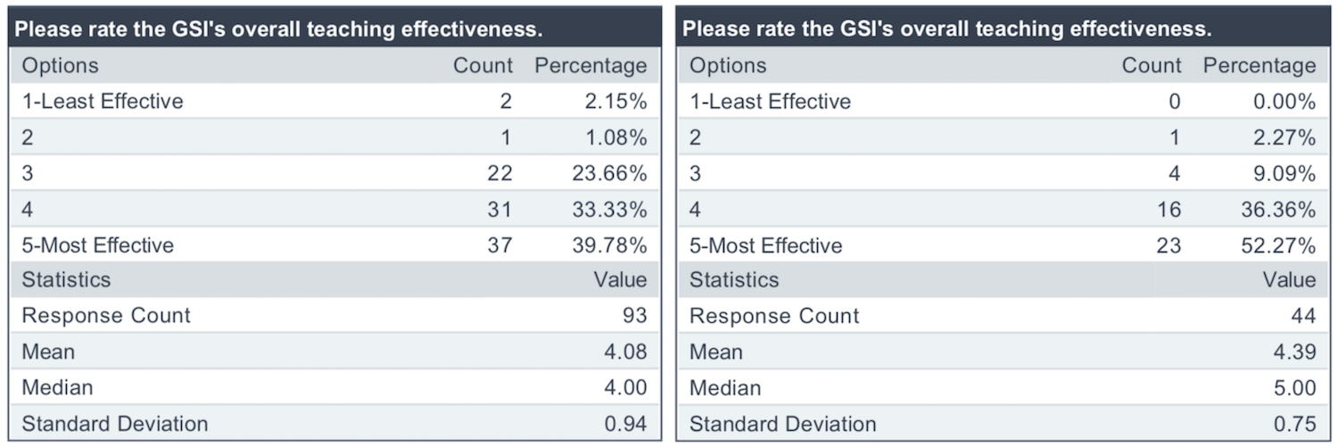
Left: undergraduate student responses. Right: graduate student responses.

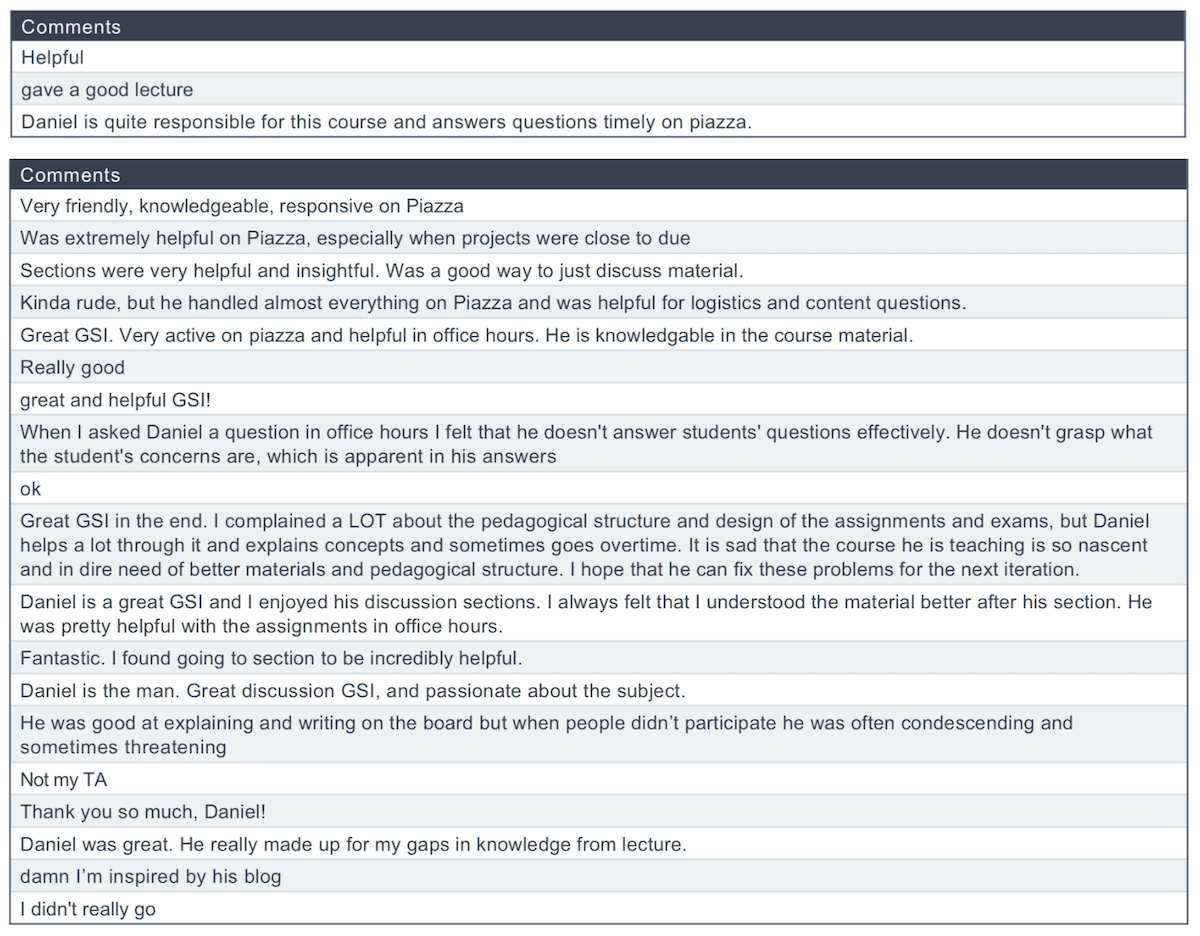
Top: graduate open-ended responses. Bottom: undergraduate open-ended responses.

My first thought was: ouch! The reviews said that the EECS department average was 4.34. Combining the undergrad and graduate ratings meant that I was below average.

Well, I was hoping to at least be remotely in contention for the Outstanding GSI award from the department. Unfortunately, I guess that will not happen. Nonetheless, I will still strive to be as effective a teacher as I can possibly be in the future. I follow the “growth mindset” from Carol Dweck,⁷ so I must use this opportunity to take some constructive criticism.

From looking at the comments, one student said I was “kinda rude” and another said I was “often condescending and sometimes threatening” (?!?!?). I have a few quick reactions to this.

• First, if I displayed any signs of rudeness, condescension, or threatening behavior (!!) in the course, it was entirely by mistake and entirely unintentional! I would be terrified if I was a student and had a course staff member threaten me, and I would never want to impose this feeling on a student.

• Regarding the criticism of “condescension,” I have tried long and hard to remain humble in that I do not know everything about every concept, and that I should not (unreasonably) criticize others for this. When I was in elementary school, one of my most painful nightmares was when a speech teacher⁸ called me out for an arrogant comment; I had told her that “skiing on black diamond trails is easy.” That shut me up, and taught me to watch my words in the future. With respect to Deep Learning, I try to make it clear if I do not know enough about a concept to help a student. For example, I did not know much about the Transformer architecture before taking this class, and I had to learn it along with the students. Maybe some of the critical comments above could have been due to vague answers about the Transformer architecture? I don’t use it in my research, unlike the three other GSIs who do, which is why I recommended that students with specific Transformer-related questions ask them.

• One possibility might be that those negative comments came from students who posted incomplete issue reports on Piazza that got my prompt response of linking to John Canny’s “filing an issue report” page (discussed earlier). Admittedly, I was probably excessively jumping the gun on posting those messages. Maybe I should not have done that, but the reality is that we simply cannot provide any reasonable help to students if they do not post enough information for us to understand and reproduce their errors, and I figured that students would want a response sooner than later.

I want to be a better teacher. If there are students who have specific comments about how I could improve my teaching, then I would like to know about it. I would particularly be interested in getting responses from students who gave me low ratings. To be clear, I have absolutely no idea who wrote what comments above; students have the right to provide negative feedback anonymously to avoid potential retaliation, though I would never do such a thing.

To any students who are genuinely worried that I will be angry at them if I get non-anonymous negative feedback from them, then in your email or message to me, be sure to paste a screenshot of this blog post which shows that I am asking for this feedback and will not get angry. Unlike Mitch McConnell, I have no interest in being a hypocrite, so I will have to take the feedback to heart. At the very least, a possible message could be structured like the following:

Dear Daniel

I was a student in CS 182/282A this past semester. I think you are a terrible GSI and I rated you 1 out of 5 on the course evaluation (and I would have given a 0 had that been an option). I am emailing to explain why you are an atrocious teacher, and before you get into a hissy fit, here’s a screenshot of your blog showing that we have permission to give this kind of feedback without retaliation:

[insert screenshot and other supporting documentation here]

Anyway, here are the reasons:

Reason 1: [insert constructive feedback here]

Reason 2: [insert constructive feedback here]

I hope you find this helpful!

Sincerely, […]

And there you have it! Without knowing what I can do to be a better teacher, I won’t be able to improve.

On the positive side, at least I got lots of praise for the Piazza comments! That counts for something. I hope students appreciated it, as I enjoy responding and chatting with students.

Obviously, if you graded me 5 stars, then thanks! I am happy to meet with you and chat over tea. I will pay for it.

Finally, without a doubt, the most badass comment above was “I’m inspired by his blog” (I’m removing the swear word here, see the footnote for why).⁹ Ha ha! To whoever said that, if you have not subscribed, here is the link.

Closing Thoughts

Whew, now that the summer is well underway, I am catching up on research and other activities now that I am no longer teaching. I hope this reflection gives an interesting perspective of a GSI for a course on a cutting-edge, rapidly changing subject. It is certainly a privilege to have this opportunity!

Throughout the semester, I recorded the approximate hours that I worked each week on this class. I’m pleased to report that my average was roughly 25 hours a week. I do not count breakfast, lunch, or dinner if I consumed them in between my work schedule. I count meetings, and usually time I spend on emails. It’s hard to say if I am working more or less than other GSIs.

Since I no longer have to check Piazza, my addiction to Piazza is now treated. Thus, my main remaining addictions to confront are reading books, blogging, eating salads, and long-distance running. Unfortunately, despite my best efforts, I think I am failing to adequately reduce the incidence of all four of these.

That is a wrap. I am still super impressed by how much John Canny is able to quickly pick up different fields. Despite being department chair in two days, he continues to test and implement his own version of the Transformer model. He will be teaching CS 182/282A next Spring, and I am told that John will try to get a better time than 8:00am, and given that he’s the department chair, he must somehow get priority on his course times. Right?

Stay tuned for the next iteration of the course, and happy Deep Learning!

I thank David Chan and Forrest Huang for feedback on earlier drafts of this post.

A photo I took of the ICRA 2019 conference banquet. Look carefully at what the performers are doing.

Last week, I attended part of the 2019 International Conference on Robotics and Automation (ICRA)¹, held in Montréal, Canada at the Palais des congrès de Montréal. I also attended ICRA 2018 last year, in Brisbane, Australia. I have blog posts which summarize my experience at ICRA 2018: the day before, day 1, day 2, day 3, day 4, and day 5. This time, I am not going to write my excessively detailed posts. First, more posts would be somewhat redundant. Second, ICRA is normally five days: workshops and tutorials are two days, while the other three are the “main” part of the conference with plenary/keynote talks and poster sessions. I was only at ICRA 2019 for the main part (May 20-22), and I prefer to write detailed summaries for when I attend a conference in its entirety. Finally, I have deadlines coming up, and my collaborators would be furious if they saw that I was spending valuable time pontificating the intricacies of ICRA rather than doing whatever they need me to do.

Of course, this post is probably on the long side anyway, but don’t tell anyone. In my defense, the majority of it was written on the return flight from the conference, and being in cramped coach class means it is nearly impossible to get real work done. Thus, this post will be structured in a similar style as my IJCAI 2018 post, except perhaps with better organization.

I was not even planning on attending ICRA 2019. I have a paper there, but my colleague Xinlei Pan at UC Berkeley is the first author and was going to present. Unfortunately, he got hit with “visa issues,” and was unable to leave the United States. As someone who happily calls himself a globalist,² this is disappointing, and I will comment on this in future blog posts.

As is my tradition for traveling, I arrived at the San Francisco International Airport early so that I could enjoy a nice dinner, followed by a long time block which allows me to read books (this is how I read so many) or assiduously work on blog posts. As evening struck that night, I boarded my red-eye Air Canada flight to Montréal.

In Montréal

Once I arrived on May 19 (the day before ICRA 2019 started), I took an Uber to the conference venue. I was there to meet the two assigned sign language interpreters, who I had been emailing and texting beforehand. I followed my pre-conference logistics checklist, and we were there to meet the venue’s employees to figure out the best seating position and the lighting situation in the lecture rooms.

Due to Xinlei’s visa situation, I only had 1.5 month’s notice for attending ICRA. Thus, Berkeley’s DSP and I had to scramble to get the logistics organized. Fortunately, DSP has been getting better and better, and was able to obtain the sign language interpreters and contact the conference organizers to get identification for them.

It was a far cry from what happened at UAI 2017. Read this blog post if you want to know the details.

The interpreters knew the American version of sign language. Since they were from Canadian cities, they were additionally able to teach me the signs for Montréal, Toronto, and Quebec. My sign language education is thus augmented by attending international conferences.

While we obtained conference badges, the lighting situation in the lecture rooms was less than ideal. It was too dark. We spoke with the relevant person in charge, and she said there was no way to fix a particular light towards a location (i.e., where the sign language interpreter would be located). I’m surprised the venue lacked that capability. At IJCAI 2018, it was easy for the venue employees to adjust the lights. I’m not sure if the Brisbane Convention Centre lecture hall has that capability, but it was brighter there so we did not have to worry.

Once I had finished discussing logistics with the sign language interpreters, I headed towards my hotel room. Or, actually, my AirBnB. I was lucky to join an AirBnB with several Berkeley students, but was unlucky with what happened two days before I arrived to Montréal: we got canceled. We were re-assigned to two different AirBnBs much farther away from the conference venue. At least the route (about a 30 minute walk) was almost entirely on one street, and seemed safe. To be honest, maybe I will just stick with hotel rooms in the future? I miss having fancy breakfasts and fitness centers, like the hotel in Sydney, Australia for UAI. That one was easily the best hotel I’ve been to for a conference, outclassing the ones from Brisbane and Stockholm.

For dinner, I got recruited by a Berkeley postdoc to eat at a famous place serving poutine. I did not know what that term meant, and upon arriving there, I realized that poutine is a dish consisting of french fries, cheese, brown gravy, and some toppings. I ordered one with grilled onions, and was able to eat all the onions. But, try as I might, I just could not eat even a fraction of the french fries. This is a popular dish associated with Quebec cuisine, but wow, how do people manage to eat this stuff?

I appreciate getting to eat poutine once. That night was my first — and last — time eating poutine.

After “dinner,” I went to a grocery store that I had the tremendous fortune to pass by. As luck would have it, there were fresh blueberries and baby carrots in stock. I bought some to eat back at the AirBnB.

I don’t think I can ever remember feeling happier to consume blueberries and baby carrots.

Day 1

On the first day of the conference, we had our opening ceremony. (This was different from Brisbane last year, when we had tutorials on the first day, followed by the opening ceremony in the evening.) There were two sets of performers: female dancers, and male singers. The dancers seemed very intense, and were impressively synchronized throughout their performance. One of the sign language interpreters commented that the applause was stronger for the male singers, who conducted a less physically strenuous task. Was there some sexism here?

After the performances, Greg Dudek gave the opening remarks. As usual, he commented on the large number of papers accepted and the growing size of the conference. Also, as usual, there was some not-so-subtle patriotism. Dudek presented the number of conference papers with respect to a country’s population, which meant Canada was in first place and ahead of the United States. Then we realized that he was half right. Canada is ahead of the United States, but not first. On the next slide, he corrected himself by showing Switzerland and Singapore in first and second place, respectively. It looks like Switzerland won the prize of papers with respect to a country’s population. Last year, Singapore won it. What happened, Singapore???

Then we had the plenary talks, followed by the keynotes. In ICRA terminology, plenaries are arguably more prestigious than keynotes, because there is exactly one plenary talk in the morning for each of the three main conference days, and this is followed by two keynotes held simultaneously.

That day, Yoshua Bengio gave the plenary talk. Oh yeah. Actually, there seem to be a lot of similarities with this year’s plenaries and last year’s:

• One famous white man: Rodney Brooks last time, Yoshua Bengio this time. Both are eminent leaders in the academic community.
• One famous man of Indian descent: Mandyam Srinivasan of Queensland last time, and Vijay Kumar of the University of Pennsylvania. Both are known for biological or aerial robots, in some sense.
• One famous white woman: Raia Hadsell of DeepMind last time, and Raquel Urtasun of Toronto/Uber. Both are famous Deep Learning researchers, and both talked about self-driving cars and navigation.
• Two out of three plenary speakers were from the conference venue’s country in some sense, either via citizenship or by working there as a permanent resident. Brooks and Srinivasan are associated with Australia, and Bengio and Urtasun are associated with Canada.

Folks, I think I see the pattern here.

Bengio’s talk was surprisingly short, and I think the reason became clear when Dudek said that Bengio had to catch a flight after his talk. I think the audience still enjoyed it, and Dudek said we could tell future generations of researchers that “we got to see Yoshua Bengio give a talk.” I don’t think that comment applied to me, because this was the second talk of his I attended; he gave one in Fall 2015 at UC Berkeley, recruited by Pieter Abbeel. That was a standing room only talk, though surprisingly, I think I remember more from that talk than from his plenary.

After Bengio’s plenary, we had poster sessions and coffee breaks. Sadly, there were no free lattes, unlike in Brisbane. Darn. In terms of the food, the coffee breaks followed a pattern of serving two main dishes: one pastry-based and one fruit-based.

ICRA 2019’s poster sessions followed the same pod-based system as last year. From browsing the topics, it was clear that deep learning, imitation learning, reinforcement learning, and autonomous driving were hot topics. Someone with more knowledge of the paper and keyword statistics might correct me on this, but my impression is that there was a similar distribution of research topics as last year.

The first set of keynote talks occurred in the afternoon. I attended the one based on industry and venture capitalism. Annoyingly, this room (not the same as the room for Bengio’s plenary) was also dark, and I did not get much benefit out of the talk as it was hard to understand the sign language interpreters. The speaker concluded with a slide that recommended six books to read. I read two out of the six: The Hard Things About Hard Things and The Lean Startup. You can see my summaries here.

After that, we had more poster sessions, and then the welcome reception in the same room. Interestingly, they limited us to two alcoholic beverages each, unlike in Brisbane where we had unlimited servings. That seems fair, as we don’t want people to overdo it. The food was also reasonable, with some intriguing smoked meat dishes and (ugh) poutine. It was cocktail-style, so I walked around sampling the food (and dessert, such as iced maple syrup) and chatting with people who I knew. Eventually, I found Ken Goldberg there with other Berkeley students, so I was able to join their group, and we took a few group photos.

After the welcome reception stopped serving food, I went back to our AirBnB. I needed to stay up late to finish some grading for CS 182/282A.³

Day 2

I woke up early to go for a run in a park near the conference venue. The trail was nice, but with respect to running routes, I give the edge to Brisbane. There was a trail underneath the highways that gave a great view of the Brisbane coastline.

I arrived to the conference venue in time for the second plenary talk, by Vijay Kumar. I was fascinated by his videos showing aerial and flying robots. And, as is typical nowadays for many robotics keynotes, Kumar talked about industry investment in robotics and AI. I left his talk thinking that I needed to (a) read some of his papers, and (b) know more about robotics-related business.

The keynotes directly followed the plenary. I chose to attend CMU Professor Matt Mason’s talk about failures in research. He was Ken Goldberg’s PhD advisor, and to the surprise of no one, Ken was sitting in the audience and taking pictures. Matt Mason was also a PhD student in the same group at MIT as John Canny was back in the 1980s. Mason and Canny were advised by the great Tomás Lozano-Pérez.⁴ It’s odd that Mason was talking about failures, because he’s had an enormously successful career. I guess that was the point!

Incidentally, it was held in the same room as the keynote from yesterday. There was more lighting near the center of the room, so the sign language interpreters and I figured out a way to position ourselves so that I could at least understand a fraction of the talk’s contents. Before the talk, we were amused when an observer told us that one of the interpreters (who was facing me) was seated in the wrong direction.

Later, for one of the poster sessions that day, I helped other members of Ken Goldberg’s lab to present the Fog Robotics paper. The metaphor of “fog” is that it’s an intermediary between the “cloud” and the “edge,” but to really understand it, read the paper. Note that Ken Goldberg is well known for cloud robotics research, and published a well-regarded survey on the topic. My colleague Ajay Tanwani was supposed to present since he is the first author, but as with Xinlei, he got snagged up with visa issues. Sigh, what in the world is going on with visa issues?

While helping to present the paper, I met someone who studies gesture recognition. She was mesmerized by the sign language interpreting, and asked to take a video of us talking (we gave permission). Meanwhile, I enjoyed describing Fog Robotics, and hope to be more involved in that research over the summer.

After the poster sessions, we had the conference banquet! Unlike in Brisbane, the conference banquet was a sit-down dinner; see the picture at the top of this post. Normally, I get into panic mode, because the most likely outcome for me is that I sit either alone or sit at a table with no one I know. At a cocktail-style dinner, I can freely move around, and if I get stuck into a conversation with someone whose utterances I cannot understand, then I can quickly (though politely!) cut ties and walk somewhere else.

As luck would have it, Ken Goldberg actually asked his lab members and lab alumni to get together right before the banquet, so that we could walk over (and, presumably, get a table). That was a HUGE relief! I think Ken anticipated this, since he told us a story about how he once got trapped into a table of strangers.

The conference banquet was amazing. Wow. It was a multiple-course dinner, and before each round of food, we had performance artists put on a show. The food included:

• Bread and butter
• Lots of wine
• Smoked salmon
• Guinea fowl (!!)
• Beet and maple yogurt
• Craquelin choux pastry

I ate everything on my plate. The quality was outstanding. The post-dessert coffee was nice because I still had to do some grading for 182/282A.

I knew people at the table I was sitting at, and we got into lively conversations about a variety of topics in robotics and automation. We wrapped up with a discussion of the economic warfare between the United States and China due to Trump’s ill-advised trade wars. I hope this is clear to readers of this post, but I am very, very anti-trade war.

To be clear, perhaps the main reason why I enjoyed the banquet was because I was actually at a table for which I knew some of the people and could participate in the conversation with the help of judiciously-placed sign language interpreters. If those attributes were not present, then my enjoyment level would have been substantially lower.

Note that this was the only main part of ICRA serving essentially an unlimited amount of alcoholic beverages. ICRA certainly did not hold back on making the banquet memorable.

Day 3

For the third main day, Raquel Urtasun gave the plenary. She went through a LOT of material quickly. Normally I am never able to follow talks of this style, but surprisingly, I think I remember more content from Urtasun’s talk than the other two plenaries. This may have been because I read Driverless: Intelligent Cars and the Road Ahead last year, so I knew some of the technical background on self-driving cars.

The second of three poster sessions today was special to me, because that was when I presented our Risk Averse Robust Adversarial Reinforcement Learning (RARARL) paper. The poster session lasted about 1.5 hours, and here is what happened:

• I tried to be active, saying “hi” to the people who came by, and shaking lots of hands. If someone was reading the poster for more than two seconds, I initiated a conversation.
• For those who I talked with, most were just asking for a general, one-minute overview of the project. Fair enough, I think this is standard.
• A handful asked for more specific details on the reinforcement learning algorithm and benchmarks that we were using.
• One person asked me why I did not have a cochlear implant.

After the poster session ended, I felt relieved, thinking that I had done as good a job as I could have. I got the “lunch box”⁵ and ate by the poster pod. Then, the sign language interpreters and I walked over to the next (and final) keynote session.

This one did not go well. The speaker’s accent was so strong that we gave up and left after five minutes. We could have tried the other keynote (remember, at ICRA, there are two keynotes per day, which happen at the same time slot), but I saw from the speaker’s name and country of origin that we would likely run into a similar problem.

Throughout the conference, I was spending lots of time looking at the sponsor exhibits. One of them was The MIT Press, which was selling books. This is my weak spot, and on the third day of the conference, I had to buy a book: The Deep Learning Revolution: Artificial Intelligence Meets Human Intelligence by Terrence J. Sejnowski. I probably know a lot of the Deep Learning history since it’s been in many other books in some form, usually along the lines of: “Hinton, LeCun, and Bengio did Deep Learning when no one else thought it was worth pursuing”. The advantage of Sejnowski’s book is understanding the perspective of a professor who performs research in this area.⁶ Sejnowski, unlike AI reporters, was actually in the subset of academia that developed Deep Learning.

We wrapped up the main part of ICRA with a farewell reception. The reception was in a smaller location than the welcome reception, and the food consisted mostly of cheese and bread dishes. Each of us got one ticket for an alcoholic beverage. The food was good, no doubt about that; I tried to get some whenever the line seemed to subside. The farewell reception was super crowded. I was only able to get a quick conversation with one person there. She was an RIT student. I introduced myself, and told her that I knew people from her school and had visited there several times. It also helped that I remembered reading her poster (about lifelong learning) at a poster session.

This year, I am sure that ICRA spent a LOT more money on the sit-down conference banquet than for the other two receptions. The conference banquet was so outstanding that the receptions, if anything, were almost a letdown. To be clear, I was not upset or disappointed in any way. This is a tradeoff that a conference has to consider. We can’t have everything in tip-top quality, because otherwise registration fees would go through the roof.

After the reception, I ate dinner at a Japanese noodle place. Then it was back to the AirBnB to finalize CS 182/282A grading. I was constantly on Slack and communicating with the other overworked GSIs for the course. We finally finished grading at 2:30AM in Eastern Standard Time.

I slept in, and when I woke up, I realized I was not in shape to go running due to exhaustion from lack of sleep over grading. I ate brunch at a unique chocolate-style cafe with “chocolate BBQ” all over the menu. I then gathered my stuff, went to the Montréal-Pierre Elliott Trudeau International Airport, bought some duty-free Swiss dark chocolate⁷ and … that was it!

Reflections

Upon leaving the conference, I graded myself as “mediocre-to-okay” with respect to networking with other attendees. I still find it very, very difficult to network at conferences, which is one of the main reasons why we have these events. It is hard to initiate conversations with people at receptions and poster sessions. There were a few times that I successfully started conversations, mostly for people who were from Berkeley. Still, for much of the poster session time, I probably spent too much time walking around aimlessly and getting food.

Overall, the food was decent at the poster sessions. I would rate the poster session food higher for Brisbane, since this year, there were too many pastries and dessert-style food. It seemed like at every poster session, the conference attendees were able to entirely finish the fruit-based dish (e.g., strawberries, melons, pineapples, etc.) but left behind much of the sweets and pastries. The banquet, though, was outstanding, and by far and away the most memorable part of the conference, and better than anything Brisbane could offer.

Last year, it seemed like there was some more governmental influence to help recruit people from the conference. We had speakers from the Australian government at ICRA. I suspect that Brisbane, and Australia more generally, has to work harder than Canada does to recruit people and stop a “brain drain.” Canada can probably recruit Americans — or foreigners educated in America — for faculty positions, and has the additional advantage of containing the origin of modern Deep Learning in Toronto.

One interesting note was that there were three people at ICRA (who I did not know beforehand) who introduced themselves to me and said that they knew about my blog. One was an incoming Berkeley PhD student, a second was a recent Berkeley PhD graduate, and a third was from somewhere else, un-affiliated with Berkeley. That was nice!

I know I am privileged in that I don’t have to worry about visa issues. I hope things will be better for students who need visas in the near future.

The sign language interpreters did a great job, and I would be happy to work with them at future conferences.

The iPhone photos I took at ICRA 2019 are hosted at my Flickr account, so that I can remember what the conference was like.

ICRA 2020 is in Paris next year. It will be interesting to see how it differs from the one in Montréal and what tradeoffs the conference organizers decide to pursue.

I will obviously do my best to get a (first-author) paper there. If so, then I promise I will write excessively detailed posts for at least all the main conference days. Stay tuned!

In my last post, I briefly mentioned that there were two relevant follow-up papers to the DQfD one: Distributed Prioritized Experience Replay (PER) and the Ape-X DQfD algorithm. In this post, I will briefly review them, along with another relevant follow-up, Kickstarting Deep Reinforcement Learning.

Distributed PER

This is the epitome of a strong empirical Deep Reinforcement Learning paper. The main idea is to add many actors running in parallel to collect samples. The actors periodically pool their samples into a centralized data repository, which is used for experience replay for a centralized learner to update neural network parameters. Those parameters then get copied back to the actors. That’s it!

Here’s what they have to say:

In this paper we describe an approach to scaling up deep reinforcement learning by generating more data and selecting from it in a prioritized fashion (Schaul et al., 2016). Standard approaches to distributed training of neural networks focus on parallelizing the computation of gradients, to more rapidly optimize the parameters (Dean et al., 2012). In contrast, we distribute the generation and selection of experience data, and find that this alone suffices to improve results. This is complementary to distributing gradient computation, and the two approaches can be combined, but in this work we focus purely on data-generation.

My first question after reading the introduction was about how Distributed PER differs from their two most relevant prior works: distributed Deep RL, also known as the “Gorila” paper (Nair et al., 2015) and A3C (Mnih et al., 2016). As far as I can tell, here are the differences:

• The Gorila paper used a distributed experience replay buffer (and no prioritization). This paper uses a centralized buffer, with prioritization. There is also a slight algorithmic change as to when priorities are actually computed — they are initialized from the actors, not the learners, so that there isn’t too much priority focused on the most recent samples.

• The A3C paper used one CPU and had multithreading for parallelism, with one copy of the environment per thread. They did not use experience replay, arguing that the diversity of samples from the different environments alleviates the need for replay buffers.

That … seems to be it! The algorithm is not particularly novel. I am also not sure how using one CPU and multiple threads compares to using multiple CPUs, with one copy of the environment in each. Do any hardware experts want to chime in? The reason why I am wondering about this is because the Distributed PER algorithm gets massively better performance on the Atari benchmarks compared to prior work. So something must be working better than before. Well, they probably used far more CPUs; they use 360 in the paper (and only one GPU, interestingly).

They evaluate their framework, Ape-X, on DQN and DPG, so the algorithms are called Ape-X DQN and Ape-X DPG. The experiments are extensive, and they even benchmark with Rainbow! At the time of the paper submission to ICLR, Rainbow was just an arXiv preprint, under review at AAAI 2018, where (unsurprisingly) it got accepted. Thus, with Distributed PER being submitted to ICLR 2018, there was no ambiguity on who the authors were. :-)

The results suggest that Ape-X DQN is better than Rainbow … with DOUBLE (!!) the performance, and using half of the runtime! That is really impressive, because Rainbow was considered to be the most recent state of the art on Atari. As a caveat, it can be difficult to compare these algorithms, because with wall clock time, an algorithm with more parallelism (i.e., Ape-X versions) can get more samples, so it’s not clear if this is a fair comparison. Furthermore, Ape-X can certainly be combined with Rainbow. DeepMind only included a handful of Rainbow’s features in Ape-X DQN, so presumably with more of those features, they would get even better results.

Incidentally, when it comes to state of the art on Atari games, we have to be careful about what we mean. There are at least three ways you can define it:

• One algorithm, applied to each game independently, with no other extra information beyond the reward signal.
• One algorithm, applied to each game independently, but with extra information. This information might be demonstrations, as in DQfD.
• One algorithm, with ONE neural network, applied to all games in a dependent manner. Some examples are IMPALA (ICML 2018), PopArt (AAAI 2019) and Recurrent Distributed PER (ICLR 2019).

In the first two cases, we assume no hyperparameter tuning per game.

In this paper, we are using the first item above. I believe that state of the art in this domain proceeded as follows: DQN -> Double DQN (i.e., DDQN) -> Prioritized DDQN -> Dueling+Prioritized DDQN -> A3C -> Rainbow -> Distributed PER (i.e., Ape-X DQN). Is that it? Have there been any updates after this paper? I suppose I could leave out the dueling architectures one because that came at the same time the A3C paper did (ICML 2016), but I wanted to mention it anyway.

Ape-X DQfD

The motivation for this paper was as follows:

Despite significant advances in the field of deep Reinforcement Learning (RL), today’s algorithms still fail to learn human-level policies consistently over a set of diverse tasks such as Atari 2600 games. We identify three key challenges that any algorithm needs to master in order to perform well on all games: processing diverse reward distributions, reasoning over long time horizons, and exploring efficiently. In this paper, we propose an algorithm that addresses each of these challenges and is able to learn human-level policies on nearly all Atari games.

The algorithm they propose is Ape-X DQfD. But, as suggested in the abstract, there are actually three main challenges they attempt to address, and the “DQfD” portion is mainly for the exploration one; the demonstrations reduce the need for the agent to randomly explore. The other algorithmic aspects do not appear to be as relevant to DQfD so I will not review them in my usual excess detail. Here they are, briefly:

• They propose a new Bellman operator with the goal of reducing the magnitude of the action-value function. This is meant to be a “better solution” than clipping rewards into $[-1,1]$. See the paper for the mathematical details; the main idea is to insert a function $h(z)$ and its inverse $h^{-1}(z)$ into the Bellman operator. I kind of see how this works, but it would be nice to understand the justification better.

• They want to reason over longer horizons, which they can do by increasing the discount factor from the usual $\gamma=0.99$ to $\gamma=0.999$. Unfortunately, this can cause instability since, according to them, it “[…] decreases the temporal difference in value between non-rewarding states.” I don’t think I understand this justification. I believe they argue that states $(x_i,a_i)$ and $(x_{i+1},a_{i+1})$ should not actually have the same value function, so in some odd sense, generalization of the value function is bad.

  To address this, they propose to add this temporal consistency loss:

  \[L_{TC}\Big(\theta; \theta^{(k-1)} \Big) = \sum_{i=1}^N p_i \mathcal{L} \Big( f_{\theta}(x_i',a_i') - f_{\theta^{(k-1)}}(x_i',a_i') \Big)\]

  with $k \in \mathbb{N}$ the current iteration number.

Now let’s get to what I really wanted to see: the DQfD extensions. DeepMind applies the following algorithmic differences:

• They do not have a “pre-training” phase, so the agent learns from its self-generated data and the expert data right away.

• They only apply the imitation loss to the best expert data. Huh, that seems to partially contradict the DQfD result which argued that the imitation loss was a critical aspect of the algorithm. Another relevant change is to increase the margin value from 0.8 to $\sqrt{0.999}$. I am not sure why.

• They use many actors to collect experience in parallel. To be precise on the word “many,” they use 128 parallel actors.

• They only use a fixed 75-25 split of agent-to-expert data.

At first, I was surprised at the last change I wrote above, because I had assumed that adding priorities to both the agent and expert data and putting them in the same replay buffer would be ideal. After all, the Ape-X paper (i.e., the Distributed Prioritized Experience Replay paper that I just discussed) said that prioritization was the most important ingredient in Rainbow:

In an ablation study conducted to investigate the relative importance of several algorithmic ingredients (Hessel et al., 2017), prioritization was found to be the most important ingredient contributing to the agent’s performance.

But after a second read, I realized what the authors meant. They still use priorities for the expert and actor samples, but these are in separate replay buffers. They are then sampled and then combined together at the 75-25 ratio. They explain why in the rebuttal:

Simply adding more actors to the original DQfD algorithm is a poor choice of baseline. First, DQfD uses a single replay buffer and relies on prioritization to select expert transitions. This works fine when there is a single actor process feeding data into the replay buffer. However, in a distributed setup (with 128 actors), the ratio of expert to actor experience drops significantly and prioritization no longer exposes the learner to expert transitions. Second, DQfD uses a pre-training phase during which all actor processes are idle. This wastes a lot of compute resources when running a decent number of actors. Many of our contributions help eliminate these shortcomings.

This makes sense. Did I mention that I really like ICLR’s OpenReview system?

The algorithm named, as mentioned earlier, is Ape-X DQfD because it uses ideas from the Ape-X paper, titled “Distributed Prioritized Experience Replay” (ICLR 2018). Yeah, more distributed systems!! I am seeing a clear trend.

What do the experiments show and suggest? Ablation studies are conducted on six carefully-selected games, and then more extensive results are reported with the same 42 (not 57) games from DQfD for which they have demonstrator data. It looks better than prior methods! Still, this is with the usual caveats that it’s near-impossible to reproduce these even if we had the same computational power as DeepMind.

In addition, with DQfD, we assume privileged information in the form of expert transitions, so it might not be fair to evaluate it with other algorithms that only get data from exploration, such as Rainbow DQN or Ape-X DQN.

After reading this paper, there are still some confusing aspects. I agree with one of the reviewer comments that the addition of demonstrations (forming Ape-X DQfD) feels like an orthogonal contribution. Overall, the paper looks like it was a combination of some techniques, but perhaps was not as rigorous as desired? Hopefully DeepMind will expand Ape-X DQfD in its own paper, as I would be interested in seeing their follow-up work.

Kickstarting Deep Reinforcement Learning

Given the previous discussion on DQfD and combining IL with RL, I thought it would be worthwhile to comment on the Kickstarting Deep Reinforcement Learning paper. It’s closely related; again, we assume we have some pre-trained “expert” policy, and we hope to accelerate the learning process of a new “student” agent via a combination of IL and RL. This paper appears to be the policy gradient analogue to DQfD. Rather than use a shared experience replay buffer, the student incorporates an extra policy distillation loss to the normal RL objective of maximizing reward. Policy distillation (see my earlier blog post about that here) cannot be the sole thing the agent considers. Otherwise, if the agent did not consider the usual environment reward, it would be unlikely to surpass performance of the teacher.

At a high level, here’s how DeepMind describes it:

The main idea is to employ an auxiliary loss function which encourages the student policy to be close to the teacher policy on the trajectories sampled by the student. Importantly, the weight of this loss in the overall learning objective is allowed to change over time, so that the student can gradually focus more on maximising rewards it receives from the environment, potentially surpassing the teacher (which might indeed have an architecture with less learning capacity).

The paper also says one of the two main prior works is “population-based training” but that part is arguably more of an orthogonal contribution, as it is about how to effectively use many agents training in parallel to find better hyperparameters. Thus, I will focus only on the auxiliary loss function aspect.

Here is a generic loss function that a “kickstarted” student would use:

where $\mathcal{L}_{\rm RL}(\omega, x, t)$ is the usual RL objective formulated as a loss function, $H(\pi_T(a | x_t) || \pi_S(a | x_t, \omega))$ is the cross entropy between a student and a teacher’s output layers, and $\lambda_k$ is a hyperparameter corresponding to optimization iteration $k$, which decreases over the course of training so that the students gradually focuses less on imitating the teacher. Be careful about the notation: $x$ implies a trajectory generated by the student (i.e., the “behavioral” policy) whereas $x_t$ is a single state. In the context of the above notation, it is a state from a teacher trajectory that was generated ahead of time. We know this because it is inside the cross entropy term.

This is a general framework, so there are more specific instances of it depending on which RL algorithm is used. For example, here is how to use a kickstarted A3C loss:

where here, $H$ is now used as simply the policy entropy (first time) of the student, and then the cross entropy (second time). As usual, $V$ is a parameterized value function which plays the role of the critic. Unfortunately, the notation for the states can be a bit confusing and conflates the student and teacher states from their respective trajectories. If I were in charge of the notation, I would use $x_t^{S}$ and $x_t^{T}$ for student and teacher states, respectively.

In practice, to get better results, DeepMind uses the Importance Weighted Actor-Learner Architecture (IMPALA) agent, which extends actor-critic methods to a distributed setting with many workers. Does anyone see a trend here?

The experiments are conducted on the DMLab-30 suite of environments. Unfortunately I don’t have any intuition on this benchmark. It would be nice to test this out but the amount of compute necessary to even reproduce the figures they have is insane.

Since it was put on arXiv last year, DeepMind has not updated the paper. There is still a lot to explore here, so I am not sure why — perhaps it was rejected by ICML 2018, and then the authors decided to move on to other projects? More generally, I am interested in seeing if we have explored the limits of accelerating student training via a set of teacher agents.

Concluding Thoughts

This post reviewed three related works to the Deep Q-Learning from Demonstrations paper. The trends that I can see are this:

• If we have expert (more generally, “demonstrator”) data, we should use it. But we have to take care to ensure that our agents can effectively utilize the expert data, and eventually surpass expert performance.

• Model-free reinforcement learning is incredibly sample inefficient. Thus, distributed architectures — which can collect many samples in parallel — result in the best performance in practice.

Imitation Learning (IL) and Reinforcement Learning (RL) are often introduced as similar, but separate problems. Imitation learning involves a supervisor that provides data to the learner. Reinforcement learning means the agent has to explore in the environment to get feedback signals. This crude categorization makes sense as a start, but as with many things in life, the line between them is blurry.

I am interested in both learning problems, but am probably even more fascinated about figuring out how best to merge the techniques to get the best of both words. A landmark paper in the combination of imitation learning and reinforcement learning is DeepMind’s Deep Q-Learning from Demonstrations (DQfD), which appeared at AAAI 2018. (The paper was originally called Learning from Demonstrations for Real World Reinforcement Learning” in an earlier version, and somewhat annoyingly, follow-up work has cited both versions of the title.) In this post, I’ll review the DQfD algorithm and the most relevant follow-up work.

The problem setting of DQfD is when data is available from a demonstrator (or “expert”, or “teacher”) for some task, and using this data, we want to train a new “learner” or “student” agent to learn faster as compared to vanilla RL. DeepMind argues that this is often the case, or at least more common than when a perfectly accurate simulator is available:

While accurate simulators are difficult to find, most of these problems have data of the system operating under a previous controller (either human or machine) that performs reasonably well.

Fair enough. The goal of DQfD is to use this (potentially suboptimal!) demonstration data to pre-train an agent, so that it can then perform RL right away and be effective. But the straightforward solution of performing supervised learning on the demonstration data and then applying RL is not ideal. One reason is that it makes sense to use the demonstration data continuously throughout training as needed, rather than ignoring it. This implies that the agent still needs to do supervised learning during the RL phase. The RL phase, incidentally, should allow the learner to eventually out-perform the agent who provided the data. Keep in mind that we also do not want to force a supervisor to be present to label the data, as in DAGGER — we assume that we are stuck with the data we have at the start.

So how does this all work? DQfD cleverly defines a loss function $J(Q)$ based on the current $Q$ network, and applies it in its two phases.

• In Phase I, the agent does not do any exploration. Using the demonstration data, it performs gradient descent to minimize $J(Q)$. DQfD, like DQN, uses an experience replay buffer which stores the demonstration data. This means DQfD is off-policy as the data comes from the demonstrator, not the agent’s current behavioral policy. (Incidentally, I often refer to “teacher samples in a replay buffer” to explain to people why DQN and Q-Learning methods are off-policy.) The demonstration data is sampled with prioritization using prioritized experience replay.

• In Phase II: the agent explores in the environment to collect its own data. It is not explicitly stated in the paper, but upon communication with the author, I know that DQfD follows an $\epsilon$-greedy policy but keeps $\epsilon=0.01$, so effectively there is no exploration and the only reason for “0.01” is to ensure that the agent cannot get stuck in the Atari environments. Key to this phase is that the agent still makes use of the demonstration data. That is, the demonstration data does not go away, and is still occasionally sampled with prioritization along with the new self-generated data. Each minibatch may therefore consist of a mix of demonstration and self-generated data, and these are used for gradient updates to minimize the same loss function $J(Q)$.

The main detail to address is the loss function $J(Q)$, which is:

where:

• $J_{DQ}(Q)$ is the usual one-step Double DQN loss.

• $J_n(Q)$ is the $n$-step (Double) DQN loss — from communication with the author, they still used the Double DQN loss, even though it doesn’t seem to be explicitly mentioned. Perhaps the Double DQN loss isn’t as important in this case, because I think having longer returns with a discount factor $\gamma$ decreases the need to have a highly accurate bootstrapped Q-value estimate.

• $J_E(Q)$ is a large margin classification loss, which I sometimes refer to as “imitation” or “supervised” loss. It is defined as

  \[J_E(Q) = \max_{a \in A}\Big[ Q(s,a) + \ell(a,a_E) \Big] - Q(s,a_E)\]

  where $\ell(a,a_E)$ is a “margin” loss which is 0 if $a=a_E$ and positive otherwise (DQfD used 0.8). This loss is only applied on demonstrator data, where an $a_E$ actually exists!

• $J_{L_2}(Q)$ is the usual $L_2$ regularization loss on the Q-network’s weights.

All these are combined into $J(Q)$, which is then minimized via gradient descent on minibatches of samples. In Phase I, the samples all come from the demonstrator. In Phase II, they could be a mixture of demonstrator and self-generated samples, depending on what gets prioritized. The lambda terms are hyperparameters to weigh different aspects of the loss function. DeepMind set them at $\lambda_1 = 1, \lambda_2 = 1$, and $\lambda_3 = 10^{-5}$, with the obvious correction factor of $\lambda_2=0$ if the sample in question is actually self-generated data.

The large margin imitation loss is simple, but is worth thinking about carefully. Why does it work?

Let’s provide some intuition. Suppose we have a dataset \(\{s_0,a_0,s_1,a_1,\ldots\}\) from a demonstrator. For simplicity, suppress the time subscript over $a$ — it’s understood to be $a_t$ if we’re considering state $s_t$ in our Q-values. Furthermore, we’ll suppress $\theta$ in $Q_\theta(s,a)$, which represents the parameters of our Q-network, which tries to estimate the state-action values. If our action space has four actions, \(\mathcal{A} = \{0,1,2,3\}\), then the output of the Q-network using the following size-3 minibatch (during training) is this $3\times 4$ matrix:

You can think of DQfD as augmenting that matrix by the margin $\ell$, and then apply the max operator to get this during the training process:

where the “max” operator above is applied on each row of the matrix of Q-values. In the above, the demonstrator took action $a_0=3$ when it was in state $s_0$, action $a_1=1$ when it was in state $s_1$, and action $a_2=2$ when it was in state $s_2$. To reiterate, this is only applied on the demonstrator data.

The loss is designed like this to make the Q-values of non-demonstrator state-action values to be below the Q-values of the state-action values corresponding to what the demonstrator actually took. Let’s go through the three possible cases.

• Suppose for a given state (e.g., $s_0$ from above), our Q-network thinks that some action (e.g., $a_0=0$) has the highest Q-value despite it not being what the expert actually took. Then

  \[Q(s_0,0) + \ell - Q(s_0,3) > \ell\]

  and our loss is high.

• Suppose for the same state $s_0$, our Q-network thinks that the action the demonstrator took ($a_0=3$ in this case) has the highest Q-value. But, after adding $\ell$ to the other actions’ Q-values, suppose that the maximum Q-value is something else, i.e., $Q(s_0,k)$ but where $k \ne 3$. Then, the loss is in the range

  \[Q(s_0,k)+\ell-Q(s_0,3) \in (0,\ell]\]

  which is better than the previous case, but not ideal.

• Finally, suppose we are in the previous case, but even after adding $\ell$ to the other Q-values, the Q-value corresponding to the state-action pair the demonstrator took is still the highest. Then the imitation loss is

  \[Q(s_0,3)-Q(s_0,3)=0\]

  which is clearly the minimum possible value.

An alternative to the imitation loss could be the cross entropy loss to try and make the learner choose the action most similar to what the expert took, but the DQfD paper argues that the imitation loss is better.

Besides the imitation loss, the other thing about the paper that I was initially unsure about was how to implement the prioritization for the 1-step and $n$-step returns. After communicating with the author, I see that probably the easiest way is to treated the 1 and $n$-step returns as separate entries in the replay buffer. That way, each of these items has independent sampling priorities.

Said another way, instead of our samples in the replay buffer only coming from tuples of the form:

in DQfD, we will also see these terms below which constitute half of the replay buffer’s elements:

This makes sense, though it is tricky to implement. Above, I’ve included the “done masks” that are used to determine whether we should use a bootstrapped estimate or not. But keep in mind that if an episode actually ends sooner than $n$ steps ahead, the done mask must be applied at the point where the episode ends!

One final comment on replay buffers: if you’re using prioritized experience replay, it’s probably easiest to keep the demonstrator and self-generated data in the same experience replay buffer class, and then build on top of the prioritized buffer class as provided by OpenAI baselines. To ensure that the demonstrator data is never overwritten, you can always “reserve” the first $K$ indices in a list of the transition tuples to be for the teacher.

The paper’s experimental results show that DQfD learns faster initially (arguably one of the most critical periods) and often has higher asymptotic performance. You can see the results in the paper.

I like the DQfD paper very much. Otherwise, I would not have invested significant effort into understanding it. Nonetheless, I have at least two concerns:

• The ablation studies seem very minor, or at least compared to the imitation loss experiments. I’m not sure why? It seems like DeepMind prioritized their other results, which probably makes sense. In theory, I think all components in the loss function $J(Q)$ matter, with the possible exception of the $L_2$ loss (see next point).

• The main logic of the $L_2$ loss is to avoid overfitting on the demonstration data. But is that really the best way to prevent overfitting? And in RL here, presumably if the agent gets better and better, it doesn’t need the demonstration data any more. But then we would be effectively applying $L_2$ regularization on a “vanilla” RL agent, and that might be riskier — regularizing RL seems to be an open question.

DeepMind has extended DQfD in several ways. Upon a literature search, it seems like two relevant follow-up works are:

• Distributed Prioritized Experience Replay, with the OpenReview link here for ICLR 2018. The main idea of this paper is to scale up the experience replay data by having many actors collect experience. Their framework is called Ape-X, and they claim that Ape-X DQN achieves a new state of the art performance on Atari games. This paper is not that particularly relevant to DQfD, but I include it here mainly because a follow-up paper (see below) used this technique with DQfD.

• Observe and Look Further: Achieving Consistent Performance on Atari. This one appeared to have been rejected from ICLR 2019, unfortunately, and I’m a little concerned about the rationale. If the reviewers say that there are not enough experiments, then what does this mean for people who do not have as much compute? In any case, this paper proposes the Ape-X DQfD algorithm, which as one might expect combines DQfD with the distributed prioritized experience replay algorithm. DeepMind was able to increase discount factor to be $\gamma=0.999$, which they argue allows for an order of magnitude more downstream reward data. Some other hyperparameter changes: the large margin value increases to $\sqrt{0.999}$, and there is now no prioritization, just a fixed proportion of student-teacher samples in each minibatch. Huh, that’s interesting. I would like to understand this rationale better.

Combining IL and RL is a fascinating concept. I will keep reading relevant papers to remain at the frontiers of knowledge.

Update May 2019: I have a blog post which describes some follow-up work in more detail.

The following consists of a set of notes that I wrote for students in CS 182/282A about adversarial examples and taxonomies. Before designing these notes, I didn’t know very much about this sub-field, so I had to read some of the related literature. I hope these notes are enough to get the gist of the ideas here. There are two main parts: (1) fooling networks with adversarial examples, and (2) taxonomies of adversarial-related stuff.

Fooling Networks with Adversarial Examples

Two classic papers on adversarial examples in Deep Learning were (Szegedy et al., 2014) followed by (Goodfellow et al., 2015), which were among the first to show that Deep Neural Networks reliably mis-classify appropriately perturbed images that look indistinguishable to “normal” images to the human eye.

More formally, image our deep neural network model $f_\theta$ is parameterized by $\theta$. Given a data point $x$, we want to train $\theta$ so that our $f_\theta(x)$ produces some desirable value. For example, if we have a classification task, then we’ll have a corresponding label $y$, and we would like $f_\theta(x)$ to have an output layer such that the maximal component corresponds to the class index from $y$. Adversarial examples, denoted as $\tilde{x}$, can be written as $\tilde{x} = x + \eta$, where $\eta$ is a small perturbation that causes an imperceptible change to the image, as judged by the naked human eye. Yet, despite the small perturbation, $f_\theta(\tilde{x})$ may behave very different from $f_\theta(x)$, and this has important implications for safety and security reasons if Deep Neural Networks are to be deployed in the real world (e.g., in autonomous driving where $x$ is from a camera sensor).

One of the contributions of (Goodfellow et al., 2015) was to argue that the linear nature of neural networks, and many other machine learning models, makes them vulnerable to adversarial examples. This differed from the earlier claim of (Szegedy et al., 2014) which suspected that it was the complicated nature of Deep Neural Networks that was the source of their vulnerability. (If this sounds weird to you, since neural networks are most certainly not linear, many components behave in a linear fashion, and even advanced layers such as LSTMs and convolutional layers are designed to behave linear or to use linear arithmetic.)

We can gain intuition from looking at a linear model. Consider a weight vector $w$ and an adversarial example $\tilde{x} = x + \eta$, where we additionally enforce the constraint that \(\|\eta\|_\infty < \epsilon\). A linear model $f_w$ might be a simple dot product:

Now, how can we make $w^T\tilde{x}$ sufficiently different from $w^Tx$? Subject to the \(\|\eta\|_\infty \le \epsilon\) constraint, we can set $\eta = \epsilon \cdot {\rm sign}(w)$. That way, all the components in the dot product of $w^T\eta$ are positive, which forcibly increases the difference between $w^Tx$ and $w^T\tilde{x}$.

The equation above contains just a simple linear model, but notice that \(\| \eta \|_\infty\) does not grow with the dimensionality of the problem, because the $L_\infty$-norm takes the maximum over the absolute value of the components, and that must be $\epsilon$ by construction. The change caused by the perturbation, though, grows linearly with respect to the dimension $n$ of the problem. Deep Neural Networks are applied on high dimensional problems, meaning that many small changes can add up to make a large change in the output.

This equation then motivated the the Fast Gradient Sign Method (FGSM) as a cheap and reliable method for generating adversarial examples.¹ Letting $J(\theta, x, y)$ denote the cost (or loss) of training the neural network model, the optimal maximum-norm constrained perturbation $\eta$ based on gradients is

to produce adversarial example $\tilde{x} = x + \eta$. You can alternatively write $\eta = \epsilon \cdot {\rm sign}\left( \nabla_x \mathcal{L}(f_\theta(x), y) \right)$ where $\mathcal{L}$ is our loss function, if that notation is easier to digest.

A couple of comments are in order:

• In (Goodfellow et al., 2015) they set $\epsilon = 0.007$ and were able to fool a GoogLeNet on ImageNet data. That $\epsilon$ is so small that it actually corresponds to the magnitude of the smallest bit of an 8 bit image encoding after GoogLeNet’s conversion to real numbers.

• In the FSGM, the gradient involved is taken with respect to $x$, and not the parameters $\theta$. Therefore, this does not involve changing weights of a neural network, but adjusting the data, similar to what one might do for adjusting an image to “represent” a certain class. Here, our goal is not to generate images that maximally activate the network’s nodes, but to generate adversarial examples while keeping changes to the original image as small as possible.

• It’s also possible to derive a similar “fast gradient” adversarial method based on the $L_2$, rather than $L_\infty$ norm.

• It’s possible to use adversarial networks as part of the training data, in order to make the neural network more robust, such as using the following objective:

  \[\tilde{J}(\theta, x, y) = \alpha J(\theta, x, y) + (1-\alpha) J\left( \theta, x + \epsilon \cdot {\rm sign}(\nabla_x J(\theta,x,y)) \right)\]

  Some promising results were shown in (Goodfellow et al., 2015), which found that it was better than dropout.

• The FGSM requires knowledge of the model $f_\theta$, in order to get the gradient with respect to $x$.

The last point suggests a taxonomy of adversarial methods. That brings us to our next section.

Taxonomies of Adversarial Methods

Two ways of categorizing methods are:

• White-box attacks. The attacker can “look inside” the learning algorithm he/she is trying to fool. The FGSM is a white-box attack method because “looking inside” implies that computing the gradient is possible. I don’t think there is a precise threshold of information that one must have about the model in order for the attack to be characterized as a “white-box attack.” Just view it as when the attacker has more information as compared to a black box attack.

• Black-box attacks. The attacker has no (or little) information about the model he/she is trying to fool. In particular, “looking inside” the learning algorithm is not possible, and this disallows computation of gradients of a loss function. With black boxes, the attacker can still query the model, which might involve providing the model data and then seeing the result. From there the attacker might decide to compute approximate gradients, if gradients are part of the attack.

As suggested above, attack methods may involve querying some model. By “querying,” I mean providing input $x$ to the model $f_\theta$ and obtaining output $f_\theta(x)$. Attacks can be categorized as:

• Zero-query attacks. Those that don’t involve querying the model.

• Query attacks. Those which do involve querying the model. From the perspective of the attacker, it is better to efficiently use few queries, with potentially more queries if their cost is cheap.

There are also two types of adversarial examples in the context of classification:

• Non-Targeted Adversarial Examples: Here, the goal is to mislead a classifier to predict any label other than the ground truth. Formally, given image $x$ with ground truth² $f_\theta(x) = y$, a non-targeted adversarial example can be generated by finding $\tilde{x}$ such that

  \[f_\theta(\tilde{x}) \ne y \quad {\rm subject}\;\;{\rm to} \quad d(x,\tilde{x}) \le B.\]

  where $d(\cdot,\cdot)$ is an appropriate distance metric with a suitable bound $B$.

• Targeted Adversarial Examples: Here, the goal is to mislead a classifier to predict a specific target label. These are harder to generate, because extra work must be done. Not only should the adversarial example reliably cause the classifier to misclassify, it must misclassify to a specific class. This might require finding common perturbations among many different classifiers. We can formalize it as

  \[f_\theta(\tilde{x}) = \tilde{y} \quad {\rm subject}\;\;{\rm to} \quad d(x,\tilde{x}) \le B.\]

  where the difference is that the label $\tilde{y} \ne y$ is specified by the attacker.

There is now an enormous amount of research on Deep Learning and adversarial methods. One interesting research direction is to understand how attack methods transfer among different machine learning models and datasets. For example, given adversarial examples generated for one model, do other models also misclassify those? If this were true, then an obvious strategy that an attacker could do would be to construct a substitute of the black-box model, and generate adversarial instances against the substitute to attack the black-box system.

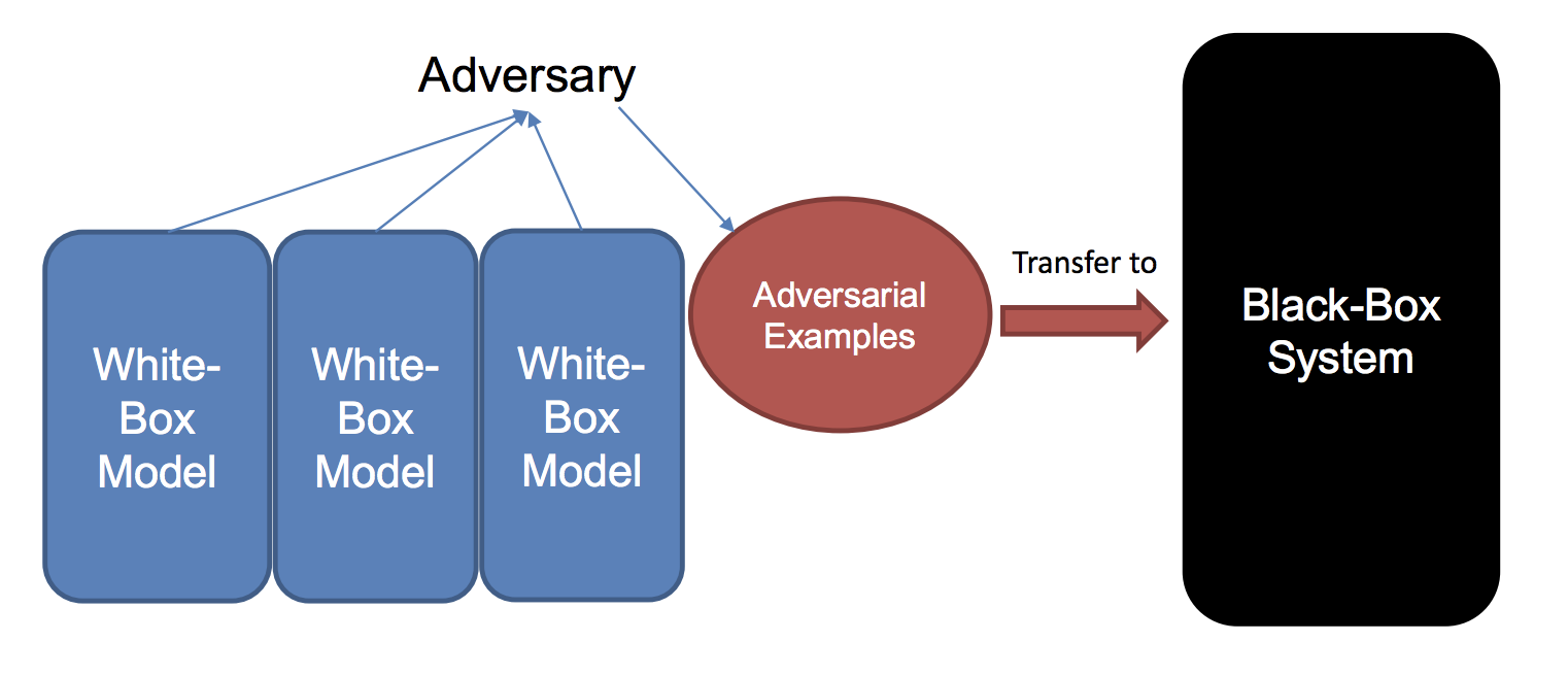
A method proposed in (Liu et al., 2017) for generating adversarial examples using ensembles.

The first large-scale study was reported in (Liu et al., 2017), which studied black-box attacks and transferrability of non-targeted and targeted adversarial examples.³ The highlights of the results were that (a) non-targeted examples are easier to transfer, which we commented earlier above, and (b) it is possible to make even targeted examples more transferrable by using a novel ensemble-based method (sketched in the figure above). The authors applied this on Clarifai.com. This is a black-box image classification system, which we can continually feed images and get outputs. The system in (Liu et al., 2017) demonstrated the ability to transfer targeted adversarial examples generated for models trained on ImageNet to the Clarifai.com system, despite an unknown model, training data, and label set.

Concluding Comments and References

Whew! Hopefully this provides a blog-post bite-sized overview of adversarial examples and related themes. Here are the papers that I cited (and read) while reviewing this content.

1. Christian Szegedy et al., Intriguing Properties of Neural Networks. ICLR, 2014.

2. Ian Goodfellow et al., Explaining and Harnessing AdversarialExamples. ICLR 2015.

3. Yanpei Liu et al., Delving into Transferable Adversarial Examples and Black-box Attacks. ICLR 2017.

The Transformer network, introduced by Google researchers in their paper titled “Attention Is All You Need” at NIPS 2017, was perhaps the most groundbreaking result in all of Deep Learning in the year 2017. In part because the CS 182/282A class has a homework assignment on Transformer networks, I finally got around to understanding some of its details, which I will discuss in this post.

Before we proceed, be aware that despite the similar-sounding names, Transformer networks are not the same thing as spatial transformer networks. Transformer networks are deep neural networks that use attention and eschew convolutional and recurrent layers, while spatial transformer networks are convolutional neural networks with a trainable module that enable increased spatial invariance to the input, which might include size and pose changes.

Introduction and Context

Way back in Fall 2014, I took CS 288 at Berkeley, which is the graduate-level Natural Language Processing course we offer. That was happening in tandem with some of the earlier post-AlexNet Deep Learning results, but we didn’t do any Deep Learning in 288. Fast forward five years later, and I’m sure the course is vastly different nowadays. Actually, I am not even sure it has been offered since I took it! This is probably because Professor Klein has been working at Semantic Machines (which recently got acquired by Microsoft, congratulations to them) and because we don’t really have another pure NLP research faculty member.

I did not do any NLP whatsoever since taking CS 288, focusing instead on computer vision and robotics, which are two other sub-fields of AI which, like NLP, heavily utilize Deep Learning. Thus, focusing on those fields meant NLP was my weakest subject of the “AI triad.” I am trying to rectify that so I can be conversationally fluent with other NLP researchers and know what words like “Transformers” (the subject of this blog post!), “ELMO,” “BERT,” and others mean.

In lieu of Berkeley-related material, I went over to Stanford to quickly get up to speed on Deep Learning and NLP. Fortunately, Stanford’s been on top of this by providing CS 224n, the NLP analogue of the fantastic CS 231n course for computer vision. There are polished lecture videos online for the 2017 edition and then (yes!!) the 2019 edition, replete with accurate captions! I wonder if the people who worked on the captions first ran a Deep Learning-based automatic speech recognizer, and then fine-tuned the end result? Having the 2019 edition available is critical because the 2017 lectures happened before the Transformer was released to the public.

So, what are Transformers? They are a type of deep neural network originally designed to address the problem of transforming one sequence into another. A common example is with machine translation (or “transduction” I suppose — I think that’s a more general umbrella term), where we can ask the network to translate a source sentence into a target sentence.

From reviewing the 224n material, it seems like from the years 2012 to 2017, the most successful Deep Learning approaches to machine translation involved recurrent neural networks, where the input source was passed through an encoder RNN, and then the final hidden state would be used as input to a decoder RNN which then provided the output sequentially. One of the more popular versions of this model was from (Sutskever et al., 2014) at NIPS. This was back when Ilya was at Google, before he became Chief Scientist of OpenAI.

One downside is that these methods rely on the decoder being able to work with a fixed-size, final hidden state of the encoder, which must somehow contain all the relevant information for translation. Some work has addressed that by allowing the decoder to use attention mechanisms to “search backwards” at earlier hidden layers from the decoder. This appears to be the main idea from (Loung et al., 2015).

But work like that still uses an RNN-based architecture. RNNs, including more advanced versions like LSTMs and GRUs, are known to be difficult to train and parallelize. By parallelize, we mean within each sample; we can clearly still parallelize across $B$ samples within a minibatch. Transformer networks can address this issue, as they are not recurrent (or convolutional, for that matter!).

(Some) Architectural Details

Though the Transformer is billed as a new neural network architecture, it still follows the standard “encoder-decoder” that are commonly used in seq2seq models, where the encoder produces a representation of the word, and the decoder autoregressively produces the output. The main building blocks of the Transformer are also not especially exotic, but rather clever arrangements of existing operations that we already know how to do.

Probably the most important building block within the Transformer is the Scaled Dot-Product Attention. Each involves:

• A set of queries \(\{q_1, \ldots, q_{n_q}\}\), each of size $d_k$.
• A set of keys \(\{k_1, \ldots, k_{n_k}\}\), each of size $d_k$ (same size as the queries).
• A set of values \(\{v_1, \ldots, v_{n_v}\}\), each of size $d_v$. In the paper, they set $d_k=d_v$ for simplicity. Also, $n_v = n_k$ because they refer to a set of key-value pairs.

Don’t get too bogged down with what these three mean. They are vectors that we can abstract away. The output of the attention blocks are the weighted sum of values, where the weights are determined by the queries and keys from a compatibility function. We’ll go through the details soon, but the “scaled dot-product attention” that I just mentioned is that compatibility function. It involves a dot product between a query and a key, which is why we constrain them to be the same size $d_k$.

Let’s stack these into matrices, which we would have to do for implementation purposes. We obtain:

where individual queries, keys, and values are row vectors within the arrays. The Transformers paper doesn’t specify the exact row/column orientation because I’m sure it doesn’t actually matter in practice; I found the math to be a little easier to write out with treating elements as row vectors. My LaTeX here won’t be as polished as it would be for an academic paper due to MathJax limitations, but think of the above as showing the pattern for how I portray row vectors.

The paper then states that the output of the self-attention layer follows this equation:

For the sake of saving valuable column space on this blog, I’ll use ${\rm Attn}$ and ${\rm soft}$ for short. Expanding the above, and flipping the pattern in the $K$ matrix (due to the transpose), we get:

In the above, I apply the softmax operator row-wise. Notice that this is where the compatibility function happens. We are taking dot products between queries and keys, which are scaled by $1/\sqrt{d_k}$, hence why we call it scaled dot-product attention! It’s also natural why we call this “compatible” — a higher dot product means the vectors are more aligned in their components.

The last thing to note for this sub-module is where the weighted sum happens. It comes directly from the matrix-matrix product that we have above. It’s easier to think of this with respect to one query, so we can zoom in on the first row of the query-key dot product matrix. Rewriting that softmax row vector’s elements as \(\{w_1^{(1)}, \ldots, w_{n_k}^{(1)}\}\) to simplify the subsequent notation, we get:

and that is our weighted sum of values. The $w_i^{(1)}$ are scalars, and the $v_i$ are $d_v$-sized vectors.

All of this is for one query, which takes up one row in the matrix. We extend to multiple queries by adding more queries as rows.

Once you understand the above, the extensions they add onto this are a little more straightforward. For example, they don’t actually use the $Q$, $K$, and $V$ matrices directly, but linearly project them using trainable parameters, which is exactly what a dense layer does. But understanding the above, you can abstract the linear projection part away. They also perform several of these in parallel and then concatenate across one of the axis, but again, that part can be abstracted away easily.

The above happens within one module of an encoder or decoder layer. The second module of it is a plain old fully connected layer:

They then wrap both the self-attention part and the fully connected portion with a residual connection and layer normalization. Whew! All of this gets repeated for however many layers we can stomach. They used six layers for the encoder and decoder.

Finally, while I won’t expand upon it in this blog post, they rely on positional embeddings in order to make use of the sequential nature of the input. Recurrent neural networks, and even convolutional neural networks, maintain information about the ordering of the sequence. Positional embeddings are thus a way of forcing the network to recognize this in the absence of these two such layers.

Experiments and Results

Since I do not do NLP research, I am not sure about what benchmarks researchers use. Hence, that’s why I want to understand their experiments and results. Here are the highlights:

• They performed two machine translation tasks: English-to-German and English-to-French. Both use “WMT 2014” datasets. Whatever those are, they must presumably be the standard for machine translation research. The former consists of 4.5 million sentence pairs, while the latter is much larger at 36 million sentence pairs.

• The metric they use is BLEU, the same one that NLP-ers have long been using for translation. and they get higher numbers than prior results. As I explained in my blog post about CS 288, I was not able to understand the spoken utterances of Professor Klein, but I think I remember him saying something like this about BLEU: “nobody likes it, everybody uses it”. Oh well. You can see the exact BLEU scores in the paper. Incidentally, they average across several checkpoints for their actual model. I think this is prediction averaging rather than parameter averaging but I am not sure. Parameter averaging could work in this case because the parameters are relatively constrained in the same subspace if we’re taking about consecutive snapshots.

• They train their model using 8 NVIDIA P100 GPUs. I understand that Transformers are actually far more compute efficient (with respect to floating point operations) than prior state of the art models, but man, AI is really exacerbating compute inequality.

• WOW, Table 3 shows results from varying the Transformer model architecture. This is nice because it shows that Google has sufficiently explored variations on the model, and the one they present to us is the best. I see now why John Canny once told me that this paper was one of the few that met his criteria of “sufficient exploration.”

• Finally, they generalize the Transformer to the task of English constituency parsing. It doesn’t look like they achieve SOTA results, but it’s close.

Needless to say, the results in this paper are supremely impressive.

The Future

This paper has 1,393 citations at the time of me writing this, and it’s only been on arXiv since June 2017! I wonder how much of the results are still SOTA. I am also curious about how Transformers can be “plugged into” other architectures. I am aware of at least two notable NLP architectures that use Transformers:

• BERT, introduced in the 2018 paper BERT: Pre-training of Deep Bidirectional Transformers for Language Understanding. It’s another Google product, but one which at the time of publication had noticeable SOTA results. You can see one of Jay Alammar’s excellent “illustrations” of it here. It looks like I have another blog added to my reading list!

• GPT-2, released in February 2019 in the form of a blog post and a preprint in ICML format (but I’m not sure if it was actually submitted to ICML, since OpenAI appears to have changed their recent publication habits). Oh yeah. Oh yeah. I have no direct comment on the controversy this created, apart from worrying that the media will continue with their click-baiting headlines that don’t accurately reveal the context and limitations of results.

I’m sure there are so many other applications of Transformers. I wonder how often Transformers have been used in robotics?

This week is UC Berkeley’s Spring Break. Obviously I’m not on vacation, because I actually need Spring Break to catch up on research due to how much time my GSI is consuming; it is taking 25-ish hours a week if I’m tracking my work hours correctly. (I’m not sure if students realize this, but teaching assistants, and probably professors, look forward to the Spring Break just as much as they do.) But I figured that since since the week would give me leeway to step off the gas pedal just a tad bit, I should use the time to tinker and improve my development environment. Broadly speaking, this means improving how I code, since my normal daily activity involves lots and lots of programming. Therefore, a proper investment in a development environment should pay for itself.

Almost two years ago, I wrote a blog post stating how I organized my GitHub repositories. That’s technically part of my development environment, but perhaps more important than GitHub repository organization is how I design my .bashrc files (or .bash_profile if I use my Mac OS X laptop) and how I organize my Python virtual environments. Those two are the subject of this blog post.

After reading my fellow lab-mate Roshan Rao’s development environment on GitHub, I realized that I was missing out on a key feature: having the git branch explicitly listed in the command line, like this where the text (master) is located after the name of this repository:

danielseita@dhcp-46-186:~/DanielTakeshi.github.io (master) $ ls 
Gemfile			_config.yml		_posts			about.md		css			new-start-here.md
Gemfile.lock		_includes		_sass			archive.md		feed.xml		subscribe.md
README.md		_layouts		_site			assets			index.html
danielseita@dhcp-46-186:~/DanielTakeshi.github.io (master) $ 

Having the branch listed this way is helpful because otherwise it is easy to forget which one I’m on when coding across multiple projects and multiple machines, and I’d rather not have to keep typing git status to reveal the branch name. Branches are useful for a variety of reasons. In particular, I use them for testing new features and fixing bugs, while keeping my master branch stable for running experiments. Though, even that’s not technically true: I’ll often make “archived” branches solely for the purpose of reproducing experiments. Finally, the value of branches for a project arguably increases when there are multiple collaborators, since each can work on their own feature and then make a pull request from their branch.

All that’s needed for the above change are a couple of lines in the .bashrc file, which I copied from Roshan earlier. No extra “plugins” or fancy installations are needed. Incidentally, I am putting my development environment online, and you can see the relevant changes in .bashrc. I used to have a vimrc repository, but I am deprecating that in favor of putting my vimrc details in the development environment. Note that I won’t be discussing vimrc in this post.

There was one annoying issue after implementing the above fix. I noticed that calling an alias which activates a virtualenv caused the git branch detail to disappear, and additionally reverted some of the .bashrc color changes. To be clear on the “alias” part, as of yesterday (heh!) I organized my Python virutual environments (“virualenvs”) by saving them all in a directory like this:

danielseita@dhcp-46-186:~ $ ls -lh seita-venvs/
drwxr-xr-x  7 danielseita  staff   224B Feb  4 21:18 py2-cs182
drwxr-xr-x  7 danielseita  staff   224B Mar  8 18:09 py2-cython-tests
drwxr-xr-x  8 danielseita  staff   256B Mar 12 21:45 py3-hw3-cs182
drwxr-xr-x  7 danielseita  staff   224B Mar  8 13:36 py3.6-mujoco
danielseita@dhcp-46-186:~ $

and then putting this in my .bashrc file:

alias  env182='source ~/seita-venvs/py2-cs182/bin/activate'
alias  cython='source ~/seita-venvs/py2-cython-tests/bin/activate'
alias hw3_182='source ~/seita-venvs/py3-hw3-cs182/bin/activate'
alias  mujoco='source ~/seita-venvs/py3.6-mujoco/bin/activate'

So that, for example, if I wanted to go to my environment which I use to test Python MuJoCo bindings, I just type in mujoco on the command line. Otherwise, it’s really annoying to have to type in source <env_path>/bin/activate each time!

But of course people must have settled on a solution to avoiding that. During the process of trying to fix the puzzling issue above of aliases “resetting” some of my .bashrc changes, I came across virtualenvwrapper, a package to manage multiple virtualenvs. I’m embarrassed that I didn’t know about it before today!

Now, instead of doing the silly thing with all the aliases, I installed virtualenvwrapper, adjusted my ~/.bashrc accordingly, and made a new directory ~/Envs in my home level directory which now stores all my environents. Then, I create virtualenvs which are automatically inserted in ~/Envs/. For example, the Python2 virtualenv that I use for testing CS 182 homework could be created like this:

mkvirtualenv py2-cs182

I often put in py2 and similar stuff to prefix the virtualenv to make it easy to remember what Python versions I’m using. Nowadays, I normally need Python3 environments, because Python2 is finally going to be deprecated as of January 1, 2020. Let’s dump Python 2, everyone!!

For Python 3 virtualenvs, the following command works for both Mac OS X and Ubuntu systems:

mkvirtualenv --python=`which python3` py3.6-mujoco

To switch my virtualenv, all I need to do is type workon <ENV>, and this will tab-complete as needed. And fortunately, it seems like this will preserve the colors and git branch changes from my .bashrc file changes.

One weakness of the virtualenvwrapper solution is that it does require a global pip installation for installing it in the first place, via:

pip install --user virtualenvwrapper

So that you can even start using it. I’m not sure how else to do this without having someone install pip with sudo access. But that should be the only requirement. The --user option means virtualenvwrapper is only applied locally to you, but it also means you have to change your .bashrc to source the local directory, not the global one. It works, but I wish there was an easy option that didn’t require a global pip installation.

As a second aside, I also have a new .bash_aliases file that I use for aliases, mostly for ssh-ing into machines without having to type the full ID, but I’ll be keeping that private for obvious reasons. Previously, I would put them in my .bashrc, but for organizational purposes, it now makes sense to put them in a separate file.

Whew. I don’t know how I managed to work without these changes above. I use multiple machines for research, so I’ll be converting all of my user accounts and file organization to follow the above.

Of course, in about six more months, I will probably be wondering how I managed to work without features XYZ … there’s just so much to learn, yet time is just so limited.

As part of my CS 182/282A GSI duties, I have been reviewing the homework assignments and the CS 231n online notes. I don’t do the entire assignments, as that would take too much time away from research, but I do enough to advise the students. Incidentally, I hope they enjoy having me as a GSI! I try to pepper my discussion sections with lots of humor, and I also explain how I “think” through certain computations. I hope that is helpful.

One reason why I’m a huge fan of CS 231n is that, more than two years ago, I stated that their assignments (which CS 182/282A uses) are the best way to learn how backpropagation works, and I still stand by that comment today. In this post, I’d like to go through the backwards pass for a 1D convolution in some detail, and frame it in the lens of matrix multiplication.

My main reference for this will be the CS 231n notes. They are still highly relevant today. (Since they haven’t been updated in a while, I hope this doesn’t mean that Deep Learning as a field has started to “stabilize” …) With respect to the convolution operator, there are two main passages in the notes that interest me. The first explains how to implement convolutions as matrix multiplication:

Implementation as Matrix Multiplication. Note that the convolution operation essentially performs dot products between the filters and local regions of the input. A common implementation pattern of the CONV layer is to take advantage of this fact and formulate the forward pass of a convolutional layer as one big matrix multiply as follows: […]

This allows convolutions to utilize fast, highly-optimized matrix multiplication libraries.

The second relevant passage from the 231n notes mentions how to do the backward pass for a convolution operation:

Backpropagation. The backward pass for a convolution operation (for both the data and the weights) is also a convolution (but with spatially-flipped filters). This is easy to derive in the 1-dimensional case with a toy example (not expanded on for now).

As usual, I like to understand these through a simple example. Consider a 1D convolution where we have input vector $\begin{bmatrix}x_1 & x_2 & x_3 & x_4\end{bmatrix}^T$ and three weight filters $w_1$, $w_2$, and $w_3$. With a stride of 1 and a padding of 1 on the input, we can implement the convolution operator using the following matrix-vector multiply:

or more concisely, $W\mathbf{x}’ = \mathbf{o}$ where $\mathbf{x}’ \in \mathbb{R}^6$ is the padded version of $\mathbf{x} \in \mathbb{R}^4$.

As an aside, you can consider what happens with a “transposed” version of the $W$ matrix. I won’t go through the details, but it’s possible to have the matrix-vector multiply be an operator that increases the dimension of the output. (Normally, convolutions decrease the spatial dimension(s) of the input, though they keep the depth consistent.) Justin Johnson calls these “transposed convolutions” for the reason that $W^T$ can be used to implement the operator. Incidentally, he will start as an assistant professor at the University of Michigan later this fall – congratulations to him!

In the backwards pass with loss function $L$, let’s suppose we’re given some upstream gradient, so $\frac{\partial L}{\partial o_i}$ for all components in the output vector $\mathbf{o}$. How can we do the backwards pass for the weights and then the data?

Let’s go through the math. I will now assume the relevant vectors and their derivatives w.r.t. $L$ are row vectors (following the CS 182/282A notation), though for the other way around it shouldn’t matter, we’d just flip the order of multiplication to be matrix-vector rather than vector-matrix.

We have:

and

Recall that in our example, $\mathbf{x} \in \mathbb{R}^4$ and $\mathbf{w} \in \mathbb{R}^3$. This must be the same shape as their gradients, since the loss is a scalar.

Notice that all the elements in the Jacobians above are from trivial dot products. For example:

By repeating this process, we end up with:

and

Upon seeing the two above operations, it should now be clear why these are viewed as convolution operations. In particular, they’re convolutions where the previous incoming (or “upstream” in CS231n verbiage) gradients act as the input, and the Jacobian encodes the convolution operator’s “filters.” If it helps, feel free to transpose the whole thing above to get it in line with my matrix-vector multiply near the beginning of the post.

Now, why does 231n say that filters are “spatially flipped?” It’s easiest to draw this out on pencil and paper by looking at how the math works out for each component in the convolution. Let’s look at the computation for $\frac{\partial L}{\partial \mathbf{x}}$. Imagine the vector $\frac{\partial L}{\partial \mathbf{o}}$ as input to the convolution. The vector-matrix multiply above will result in a filter from $\mathbf{w}$ sliding through from left-to-right (i.e., starting from $\frac{\partial L}{\partial o_1}$) but with the filter actually in reverse: $(w_3,w_2,w_1)$. Technically, the input actually needs to be padded by 1, and the stride for the filter is 1.

For $\frac{\partial L}{\partial \mathbf{w}}$, the filter is now from $\mathbf{x}$. This time, while the filter itself is in the same order, as in $(x_1,x_2,x_3,x_4)$, it is applied in reverse, from right-to-left on the input vector, so the first computation is for $\frac{\partial L}{\partial o_4}$. I assume that’s what the notes mean as “spatially flipped” though it feels a bit misleading in this case. Perhaps I’m missing something? Again, note that we pad 1 on the input and use a stride of 1 for the filter.

In theory, generalizing to 2D is, as Professor John Canny has repeated said both to me individually and the CS 182/282A class more broadly, just a matter of tracking and then regrouping indices. In practice, unless you’re able to track indices as well as he can, it’s very error-prone. Be very careful. Ideally this is what the CS 182/282A students did to implement the backwards pass, rather than resort to looking up a solution online from someone’s blog post.